Frequency response of distributed constant circuit

Figure 1 shows the expression for the frequency response of a distributed constant circuit.

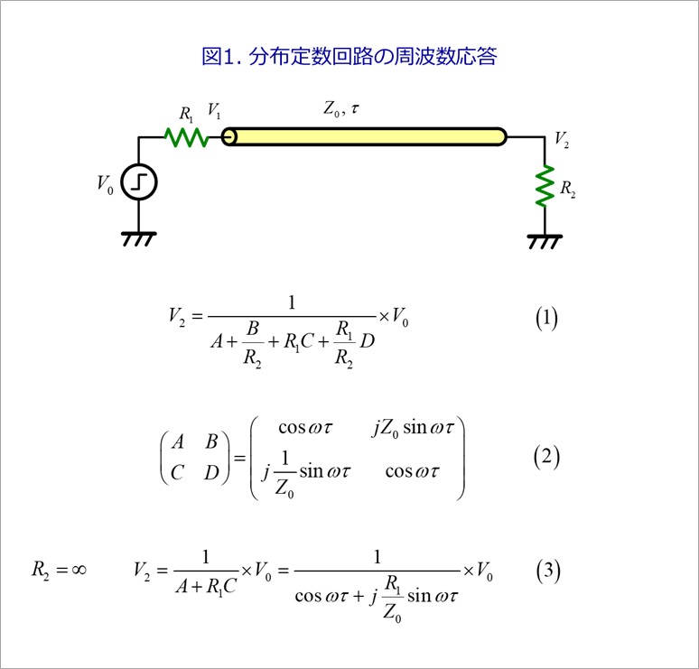
To find the far-end voltage V2, it is convenient to use a cascade.
Equation (1) in the same figure is the voltage V2 at the far end using a cascade.
A vertical row is shown in equation (2). References (1)
Since normal CMOS is open at the far end, R2 = ∞.

The simplest form of signal source V0 in Figure 2 is the trapezoidal wave shown in Figure 2.

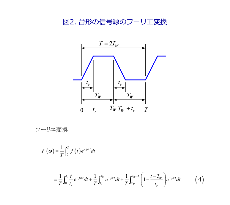
The frequency function of this trapezoidal wave is orthodoxly obtained by dividing it into the rising portion, flat portion, and falling portion and performing the Fourier transform as shown in equation (4) in Fig. 2.
The 1st and 3rd terms on the right side are calculated using partial integration, but it is more complicated than I thought.

In fact, the shape of the integral is similar between the Laplace transform and the Fourier transform. The Laplace transform is relatively easy to calculate because it uses a formula instead of integrating each time. After the Laplace transform, set s=jω and divide by the interval of integration to get the Fourier transform.

The Fourier transform and the Laplace transform are fundamentally different.
If you explain it mathematically, there will be a lot of troublesome things, but from the standpoint of a circuit maker, I think it's safe to say that the two are like relatives.
Mathematicians are likely to scold me.

The Laplace transform of the trapezoidal wave in Figure 2 can be obtained easily enough to be expressed in one line, as shown in Equation (5) in Figure 3.

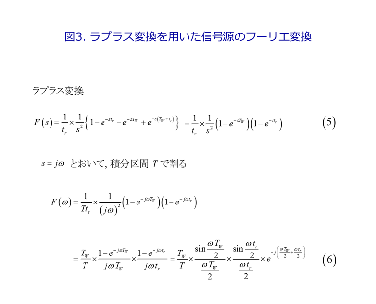
This equation (5) is the addition and subtraction of the time delay of the ramp waveform (1/s^2).
The frequency function can be easily obtained by dividing the result of the Laplace transform by the integration interval T with s=jω as shown in equation (6). Naturally, equations (4) and (6) are the same.

Time (step) response of distributed constant circuit

If V0 in Figure 1 is F(ω) in Figure 3, the voltage V2 at the far end is given by Equation (7) in Figure 4.

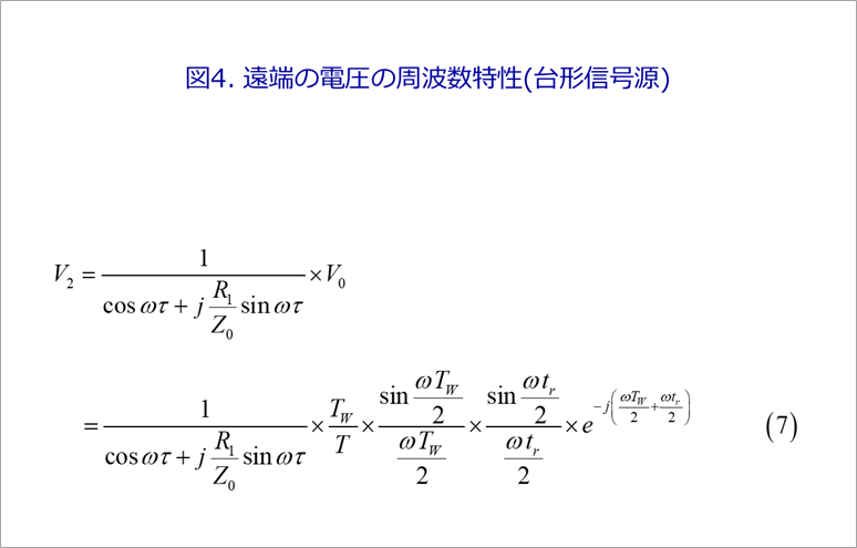
Equation (7) is a function of ω, and the inverse Fourier transform gives the time function v2(t).

The above is to find the time response by performing frequency analysis and inverse Fourier transform. next,

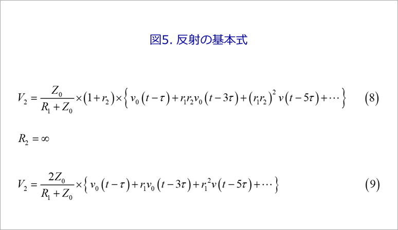
Equation (8) in Figure 5 is the basic equation for finding the far-end voltage due to repeated reflections. References (2)
In the case of CMOS transmission, since R2 = ∞, r2 = 1, which is somewhat simpler as shown in equation (9).

Figure 6 shows the case where v0(t) in Equation (9) in Figure 5 is a step waveform with an amplitude of 1.

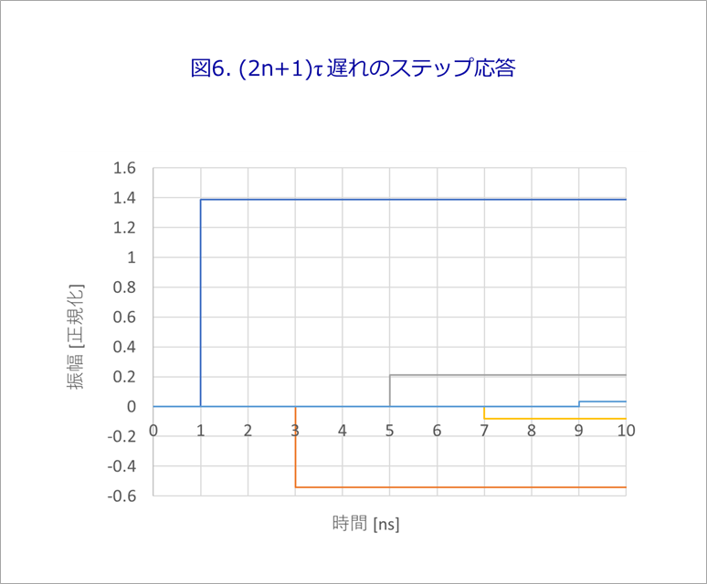
Assume that R1=22Ω, Z0=50Ω, and the line delay time τ is 1ns.
After a delay of τ(1ns), the first amplitude of 2Z0/(R1+Z0) appears, followed by another 2τ, that is, the amplitude multiplied by the near-end reflection coefficient r1 (=-0.389) with a delay of 3τ, then 5τ, 7τ. , ...(2n+1)τ and each waveform is delayed by an odd multiple of τ.

Figure 7 is a summation of waveforms delayed by odd multiples of τ from Figure 6. This is the far end voltage V2.

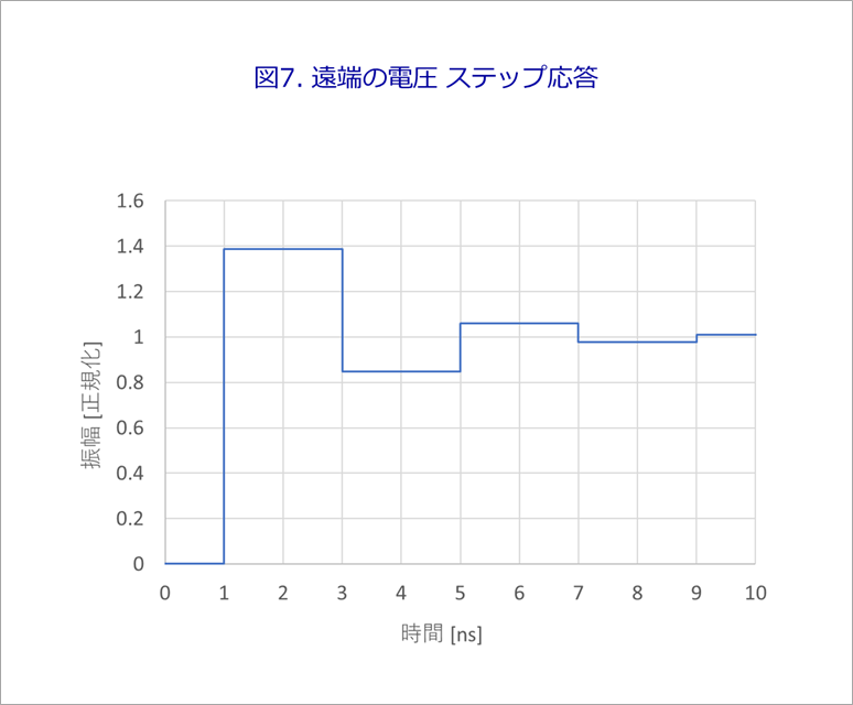
The above step response is useful for understanding how reflection works, but the actual waveform has a slope.

Overlay with ramp waveform

A waveform with a finite slope (ramp waveform) is analyzed in the same way instead of a step response.

Figure 8 is a ramp waveform similar to Figure 6.

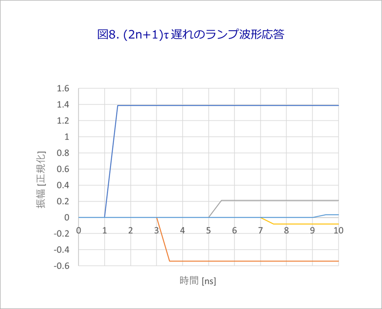
Figure 9, like Figure 7, is a summation of waveforms delayed by odd multiples of τ in Figure 8.

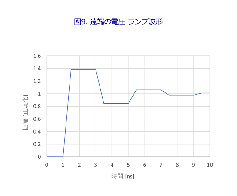
A little closer to the actual waveform.

Step waveform + Bessel filter waveform

Next, the waveform obtained by passing the step waveform through the Bessel filter, which is the purpose of this article, is used as the signal source.

See below.
Difference between Bessel filter and other filters Part 2

Figure 11 in this article is a waveform when a step waveform is passed through a Bessel filter.
The figure shows a 7th-order low-pass filter LPF (LPF: Low-Pass Filter).
Please refer to Figure 12 (a) to (c) for the waveforms of the rising portion due to the difference in the order of the filter.

They are normalized to a cutoff frequency fc of 1.
Equation (10) in Figure 10 is the transfer function F(s) of the 3rd order Bessel filter.

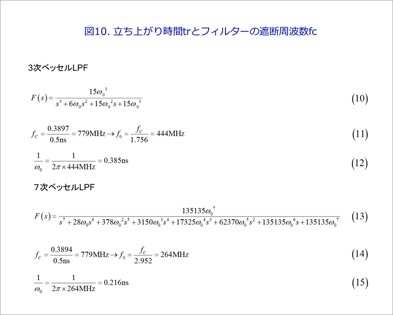
The product of 0%-100% rise time tr and fc when a step waveform is applied to this filter is fc×tr=0.3897, as shown in equation (11) for the 3rd order Bessel LPF. Therefore, if tr=0.5ns, then fc=0.3897/0.5ns=779MHz, and for 3rd order Bessel, f0=fc/1.756=444MHz.

Running through an LPF introduces delay.
The delay of a Bessel filter is approximately the group delay, which is 1/ω0.
For 3rd order Bessel, 1/ω0 is 0.385ns as shown in equation (12).

The 7th-order Bessel transfer function is Equation (13).
Similar to the 3rd order, fc and f0 are shown in equation (14).
The group delay is 1/ω0=0.216ns as shown in equation (15).

These delays occur when passing through Bessel, so this delay must be taken into account in order to start up at time t=0.

Time response (inverse Laplace transform)

The step response of the Bessel LPF is obtained by inverting the Lapsler by multiplying the transfer function by 1/s of the step waveform.

Equation (16) in Figure 11 adds a step waveform to the Bessel 3rd order LPF.

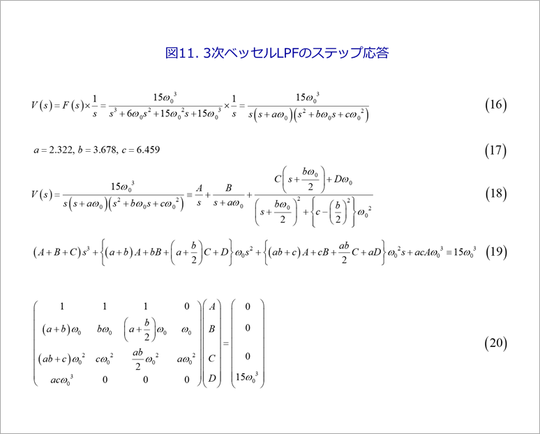
The right side of the equation is the denominator factored into the product of the linear and quadratic expressions.

To find the inverse Laplace transform of equation (16), expand it into partial fractions as in equation (18).
The numerator of the third term on the right side of the equation can be simply Cs+D, but in order to facilitate the inverse Laplace transform, C and D are multiplied by a coefficient as shown in the equation. References (3)

The unknown coefficients A through D in equation (18) are converted to identities with respect to s by removing the denominator of the equation and comparing the coefficients for each power of s on the right and left sides.
Since the right side is only a constant term, the coefficients of powers of s on the left side are all 0 (zero).
Formula (20) is a system of these equations, which is solved to find A to D and then Laplace transform them.

Equations (21) and (22) in Figure 12 are transformed into cosine and sine by the Laplace inverse transform of the third term on the right side of Equation (18). Both include an exponential decay term. References (3)

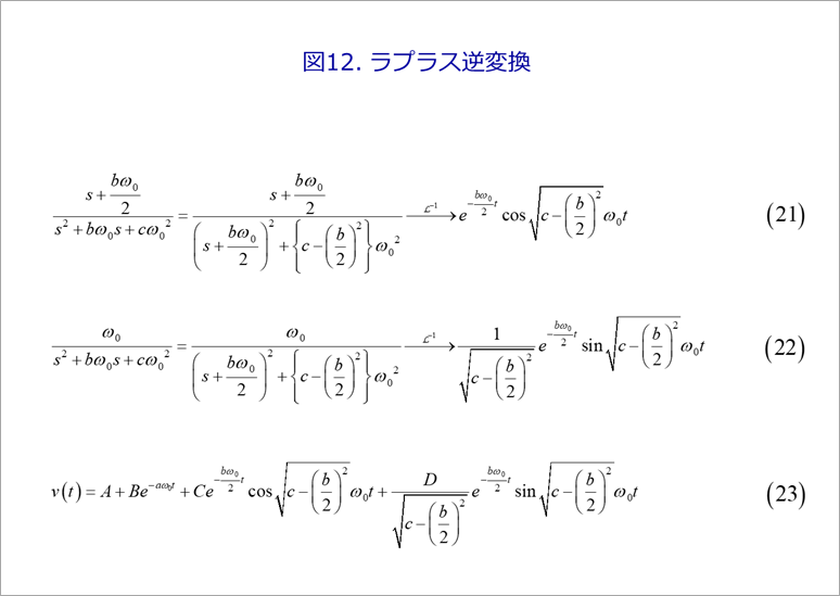
Equation (23) is the result of inverse Laplace transform.

Figure 13(a) shows the rising part of equation (23).

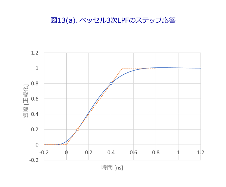
Simultaneously shows the ramp waveform connecting the 20% and 80% points of the rise with a straight line.
These are for the 3rd-order Bessel LPF, but the 7th-order LPF, for example, can be obtained in the same way, albeit a little more complicated.
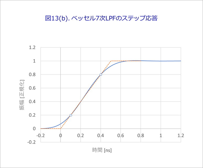
The 7th order corresponding to Equation (16) can be factored into 1st order and 2nd order × 3 denominators.
As with equation (20), set up simultaneous equations and find the unknown coefficients.
The results are shown in Figure 13(b). It can be seen that the 20%-80% part is closer to a straight line than the third order.

Based on the waveform in Fig. 13(b), calculate the reflected waveform, and find the waveform at each timing as shown in Fig. 14, just like Fig. 6 and Fig. 8.

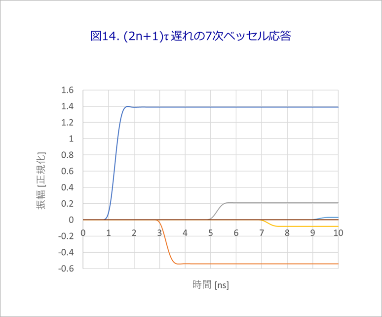
Fig. 15 shows the waveforms of Fig. 14 overlaid on the time axis, and we were able to obtain a waveform close to the actual reflected waveform.

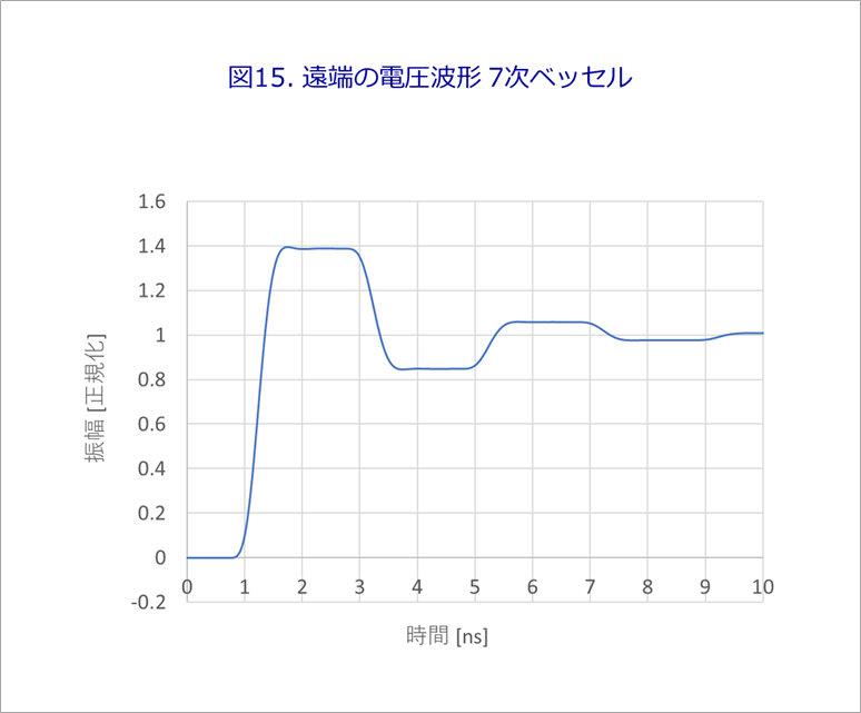
This is similar to the analysis method using Waveform data of IBIS.
See below.

Analysis of Reflection Using IBIS Model - Part 2

References
(1) Yuzo Usui : "All About Distributed Constant Circuits for Board Designers, 3rd Edition" Self-published, 2016 (http://radioy.a.la9.jp/book/book.htm), pp.156- 158

(2) Ibid., pp.20-43

(3) Ibid., p.232