Bergeron Analysis

In "Analysis of Reflection Using the IBIS Model - Part 1", we obtained the static characteristics of the driver's output. We will use this to analyze reflections. Bergeron analysis is used for this purpose. Bergeron is the name of a French engineer, and the method was originally devised for the analysis of water hammer in dams. It is used not only for transient analysis of distributed parameter circuits, but also for water hammer and acoustic analysis.

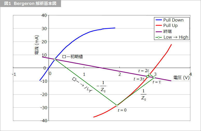
Figure 1 is a basic diagram of Bergeron analysis used for transient analysis of distributed parameter circuits. Provide the voltage-current characteristics of the driver and receiver and the characteristic impedance of the line.
In the figure, (a) is the pull-down characteristic of the driver, and (b) is the pull-up characteristic. (c) is the characteristics of the receiver, which is usually open since it is CMOS, but can be analyzed even with termination resistors and nonlinear clamp diodes.
IBIS lists Typ, Min and Max, but it seems that only Typ is usually used for transient characteristics.

Concrete example

The analysis procedure is described using Fig. 1. The blue and red lines are the pull-down and pull-up characteristics obtained in "Analysis of Reflection Using the IBIS Model - Part 1". The purple downward-sloping straight line is the termination resistor connected to the receiver end. Since it is normally open, it matches the horizontal axis, but for explanation purposes, the resistance value is 200 Ω and the termination voltage is 1.5 V. As for the direction of the current, the direction that flows into the driver is positive. Therefore, it can be seen from the figure that when the driver is at a low voltage level, current flows into the driver, so the current is positive, and when it is at a high voltage level, it is negative. The intersection of the Pull-Down and Pull-Up curves with the terminating resistor is the initial low and high value.
The figure shows step-by-step how to analyze the transition from low to high.

1. Draw a downward-sloping straight line of the characteristic impedance from the low initial value. Since the vertical axis is current and the horizontal axis is voltage, it is -1/Z0.
2. The intersection with the Pull-Up curve is the first level at t = 0.
3. From this point, draw an upward-sloping straight line of the characteristic impedance.
4. The intersection with the termination resistor is the voltage on the receiver side at t = τ (τ: tau, lowercase Greek letter).

以下同様に、交互に直線の傾きを正負に変更して、交点を求めます。
図の例では、t ＝ 3τ でほぼ振幅は落ち着いています。

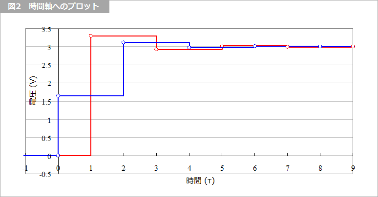
The intersection with this pull-up is the amplitude of the driver, and the intersection with the terminating resistor is the amplitude of the receiver. The change from high to low can be determined similarly.

transient characteristics

So far, we have discussed static characteristics and how to use them, including "Analysis of Reflection Using IBIS Model - Part 1". IBIS also describes transient characteristics.
One represents voltage over time in the form of the Ramp characteristic shown in Table 1.

[Ramp]

|dV/dt_r

9.900e-001/2.939e-010

7.782e-001/3.682e-010

1.142e+000/2.496e-010

dV/dt_f

8.856e-001/3.829e-010

6.654e-001/4.490e-010

1.043e+000/3.405e-010

R_load = 50ohms

Table 1 Ramp data

In the table, dV/dt_r indicates rise and dV/dt_f indicates fall, respectively, and they are listed in order of Typ, Min, and Max, just like the static characteristics.
For example, 9.900e-001/2.939e-010 listed for rising in Table 1 means a change of 0.99 V per 0.2939 ns, but this 0.99 V means an amplitude of 20% to 80% of full amplitude. To do.

The other is the waveform data shown in Table 2.

[Rising Waveform]

R_fixture = 50

V_fixture = 0

V_fixture_min = 0

V_fixture_max = 0

| time

V (typ)

V (min)

V (max)

|

0.0000e+000

0.0000e+000

0.0000e+000

0.0000e+000

8.3333e-011

0.0000e+000

0.0000e+000

0.0000e+000

1.6667e-010

7.1110e-007

2.8449e-009

2.5183e-006

2.5000e-010

2.8350e-006

2.4680e-006

1.6760e-006

4.4167e-009

1.6500e+000

1.2970e+000

1.9030e+000

4.5000e-009

1.6500e+000

1.2970e+000

1.9030e+000

4.5833e-009

1.6500e+000

1.2970e+000

1.9030e+000

4.6667e-009

1.6500e+000

1.2970e+000

1.9030e+000

4.7500e-009

1.6500e+000

1.2970e+000

1.9030e+000

4.8333e-009

1.6500e+000

1.2970e+000

1.9030e+000

4.9167e-009

1.6500e+000

1.2970e+000

1.9030e+000

5.0000e-009

1.6500e+000

1.2970e+000

1.9030e+000

Table 2 Waveform data

The first column represents the time, and the next three columns represent the typical (Typ), minimum (Min), and maximum (Max) voltages. Therefore, if we represent the waveform as a line, the full amplitude is 0.99 ÷ 0.6 = 1.65 V.
 
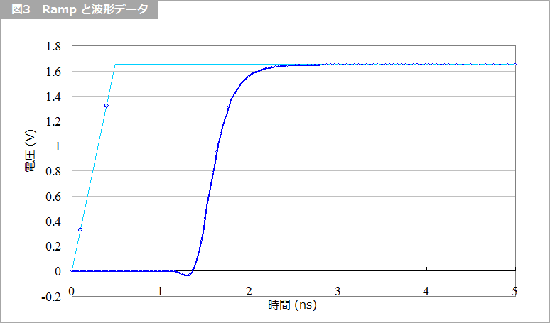
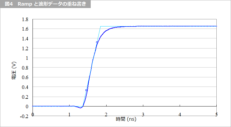
Figure 3 shows Ramp and waveform data plotted on the same graph. Waveform data includes delay time, so if you superimpose Ramp on the waveform data as shown in Figure 4, you can understand the relationship between the two.

Let's apply this Ramp characteristic and waveform data to the Bergeron analyzed waveform.

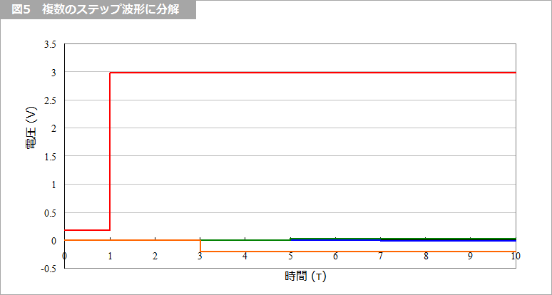
Figure 5 decomposes the far-end waveform of Figure 2 into multiple stepped waveforms. The horizontal axis of the figure shows the delay time τ of the line from the driver to the receiver.
The board delay time is about 6.5 ns/m, so if the wiring length is 10 cm, τ = 0.65 ns.

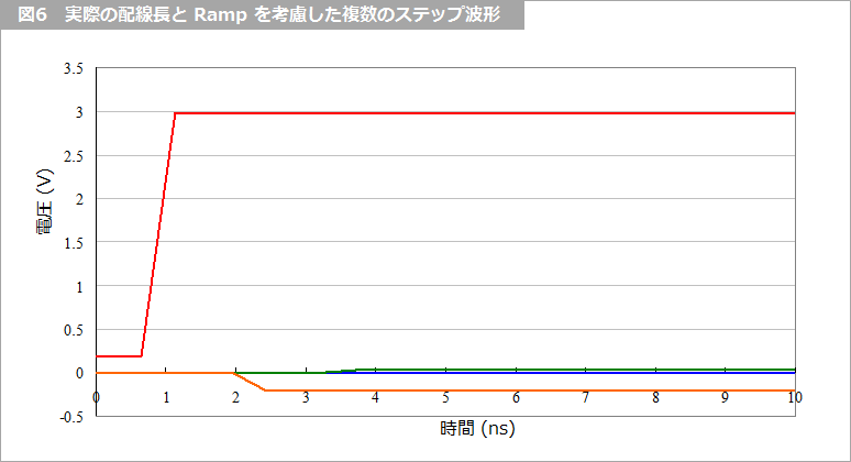
Figure 6 is obtained by replacing each step waveform of Figure 5 with the Ramp waveform of Figure 3, with one scale of the horizontal axis of Figure 5 set to 0.65 ns.

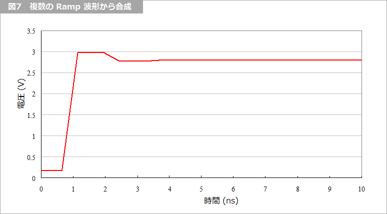
Figure 7 is a composite of the Ramp waveforms of Figure 6 added together. You can see that it is closer to the actual waveform than Fig.2.

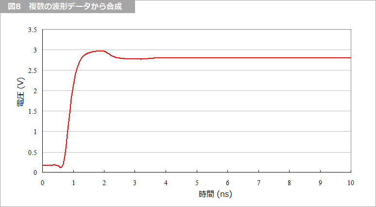
Fig. 8 shows the step waveform replaced with waveform data, and the waveform can be obtained as smoothly as the actual waveform.

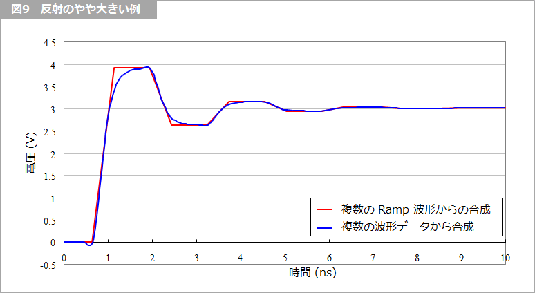
Figure 9 shows an example of large reflections, synthesized from the Ramp waveform and synthesized from the waveform data, overlaid for a little clarity.

These waveforms can be obtained using IBIS with many waveform analysis software, so it may not be possible to actually obtain them by combining Bergeron analysis and Ramp waveforms or waveform data. If you understand how it will be used, I think analysis software will look a little different from a mere black Box. Please understand how it works.