The Laplace and Fourier transforms have been previously mentioned below.

Laplace transform and Fourier transform

The advantages and disadvantages of both are described in the column above, but if I repeat it again,

Advantages and disadvantages of the Laplace transform
Pros: Easy conversion and inverse conversion using conversion formulas
Disadvantage: Can't convert if it doesn't apply to the formula → need to devise to apply to the formula

Advantages and Disadvantages of the Fourier Transform
Advantages: Numerical calculations can be easily performed using FFT
Disadvantage: Periodic function is required → It is not fatal because it is sufficient to set the period

It looks like.

As for the Fourier transform, I have already discussed the FFT in two parts in this column.

FFT by Excel
FFT by Excel (Part 2)

See below for the frequency characteristics of distributed constant lines.

Frequency characteristics of distributed constant line
Frequency characteristics of distributed parameter lines continued

Let's compare the Laplace transform and the Fourier transform.

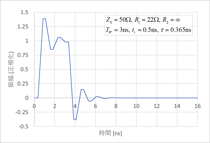
Figure 1 is an example of a reflected waveform. The driver output resistance R1 = 22Ω, corresponding to a 12mA driver. This is an example of a slightly large reflection. Assume a pulse width of 3 ns, a driver signal rise time of 0.5 ns (0%-100%), and a line delay time of 0.365 ns, approximately 5 cm.

If you transform the same circuit with Laplace and Fourier and strictly compare the difference between the waveforms of both, you can see the difference. However, this difference is a theoretical difference and does not pose a problem in practice. However, please understand that it is a technique that can be applied when you encounter similar comparisons.

The FFT sampling point N is chosen to be a power of 2, usually around 256 or 1,024, but here we choose a fairly large 16384 (2 to the 14th power) points to reduce the effect of N. The transform from time to frequency is called the Fourier transform FFT, and vice versa, the transform from frequency to time is called the inverse Fourier transform iFFT.

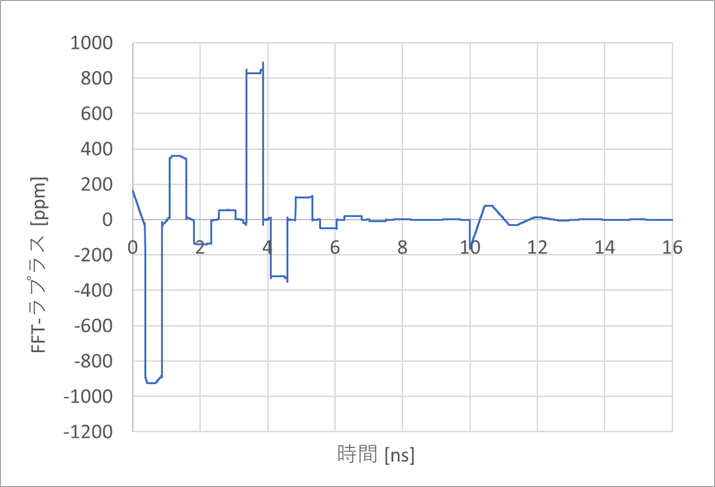
Figure 2 plots the difference between the iFFT and Laplace transform waveforms. The difference is small, so the vertical axis is expressed in ppm. This difference is small, not reaching 1,000ppm (0.1%) at most.

The reason for this difference is that Laplace is a transient and Fourier is a periodic function. In other words, the phenomenon of the Laplace transform starts at time zero (0). On the other hand, in the Fourier transform, the phenomenon continues with the same cycle all the time. Even if the reflected waveform seems to have stopped, the reflection continues, albeit slightly.

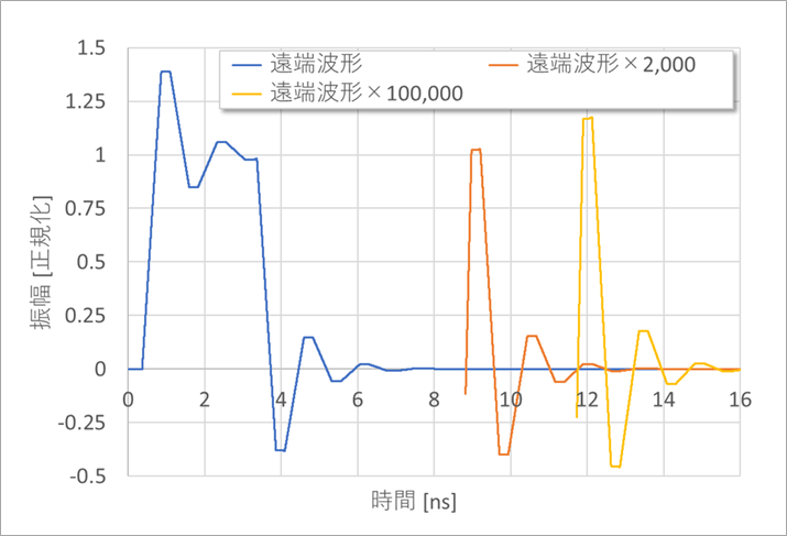
Figure 3 shows an enlarged view of the part of the reflected waveform where the reflection seems to have stopped. Magnification of 2,000 times after around 9 ns shows that the reflection still continues, and furthermore, after around 12 ns, if you multiply by 100,000, you can see that the reflection continues. Remnants of reflections that appear at times of 2,000 or 100,000 are not really a problem, but be aware of the difference between transients and repetitive waveforms.

In order to compare Laplace and Fourier on an equal footing, one cycle T of the Fourier transform is superimposed on the Laplace transform starting at time 0 and the Laplace transform starting at time T to create a pseudo periodicity.

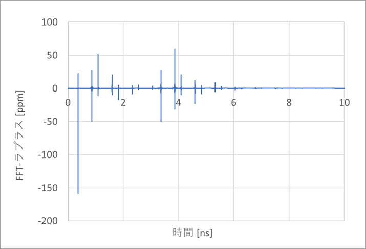
Figure 4 plots the difference between the second period of the Laplace transform and the 16,384-point iFFT. In the same figure, small reflections that seem to have settled in Fig. 3 are taken into account, so the difference like in Fig. 2 disappears, but a new acicular error appears.

What is the cause of this acicular error?

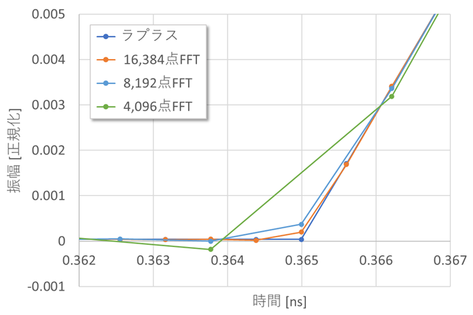
The largest difference in Figure 4 is the first rise. Figure 5 shows an enlarged view of the Fourier and Laplace analysis results in this area. Figure 4 shows iFFT with N=16,384 points as mentioned above, but Figure 5 shows N=16,384, N=8,192 and N=4,096. The smaller N, the greater the difference from Laplacian.

Here, Laplace is analyzed with a polygonal line. Since the bends of the line have high frequency components, iFFT needs a very large N to faithfully analyze them. A broken line is useful for explaining the principle, but the actual waveform changes smoothly. The comparison of smooth waveforms will be discussed later.