FFT

The Fourier transform can literally be calculated at high speed using FFT (Fast Fourier Transform).

FFT requires sample points to be chosen to be powers of two. The concept of FFT was invented in 1965. At that time, the power of computers was still low, and it took about 20 years before it came into practical use. However, at that time, it was necessary to use a dedicated LSI for high-speed processing, and in my experience, it was necessary to add a hardware option for high-speed operation to the workstation in order to perform processing with software. I remember it taking a few minutes.

FFT by Excel

Now, it's built into Excel, allowing instant calculations even on not-so-fast PCs.

FFT is the transformation of a time function into a frequency function, and its inverse is called iFFT (inverse FFT). The Excel add-in performs batch processing, but the FFT algorithm is easy to understand, so if you assemble it yourself, real-time processing becomes possible relatively easily.

This section describes how to use add-ins. As an example, use the pulse waveform described in "Laplace Transform and Fourier Transform".

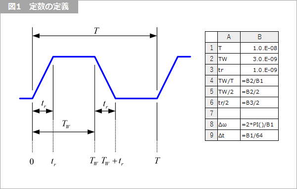
First, define the constants as shown in Figure 1. In the example, period T=10ns, pulse width TW=3ns, rise time tr=1ns. Find the increment (step) of the angular frequency ω in B8. The increment frequency is 1/T, so Δω=2π/T. Enter the time interval for iFFT processing in B9. The increment is the period divided by the number of samples N in the FFT, i.e. Δt=T/N. In this example, N=64.

• π:: lowercase greek letter pi
• ω: Greek lowercase omega

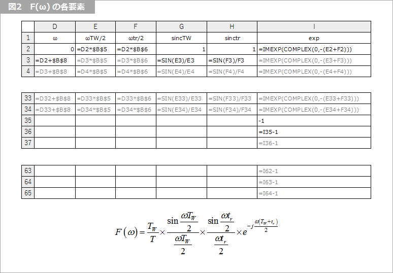
Figure 2 shows the elements of F(ω). Column D is ω, in increments of 0 to Δω. There are 64 rows in total. Gray-colored cells copy the cells above them downwards. The same is true for subsequent columns. Column E is ωTW/2 and column F is ωtr/2. Column G is the sinc function of ωTW/2, i.e. sin(x)/x. Similarly, column H is the sinc function of ωtr/2. Since sinc(0)=1, the line with ω=0 is set to 1. Column I is exp{-jω(TW+tr)/2} . The complex exponential function is imexp. From column D to column I, 33 calculations are performed for rows 2 to 34. It is N/2+1. Below I35 is the index for the wrap calculation.

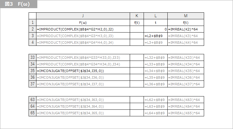
Figure 3 is F(ω). The overall coefficient is TW/T of B4, multiplied by two sinc functions (columns G and H), converted to complex numbers by the complex function, and multiplied by the exponent (column I) by the improduct function. (Column J) F(ω) finds positive and negative ω. J2 is DC and J3 through J34 are positive ω. Negative ω is the complex conjugate of F(ω) of positive ω, so find the complex conjugate symmetrically about J35. The index for that is from I35 down. J35 is offset($J$35, I35), find -1 of J35, ie J34, and find its complex conjugate with the imconjugate function. Towards the bottom, the negative number of offset increases by one, so J36 finds -2 of J35, ie J33, and finds the complex conjugate. Find J65 in the same way.

Now that we have F(ω), we can compute iFFT(F(ω) to f(t)).

Preparing Excel (add-in)

To use FFT/iFFT, you need to add a Fourier analysis add-in to Excel. How to do that depends on your version of Excel.

Older versions (2003 and older)
[Preparation]

• Check Tools -> Add-ins -> Analysis Tools

[analysis]

• Tools → Analysis Tools → Fourier Analysis

Newer versions (2007 and newer)
[Preparation]

• File -> Options -> Add-Ins -> Manage Excel Add-In Settings -> Check Analysis Tools

[analysis]

• data → data analysis → Fourier analysis

Fourier analysis

Both versions are almost the same after the above "Fourier analysis".
Source $J$2:$J$65
Destination $K$2
Check for reverse conversion

This will output the time function (complex number with 0 imaginary part) on K2:K65. Extract the real part of column K into column M for graphing. The time axis is the L column, and the increment is Δt of B9.

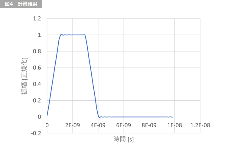
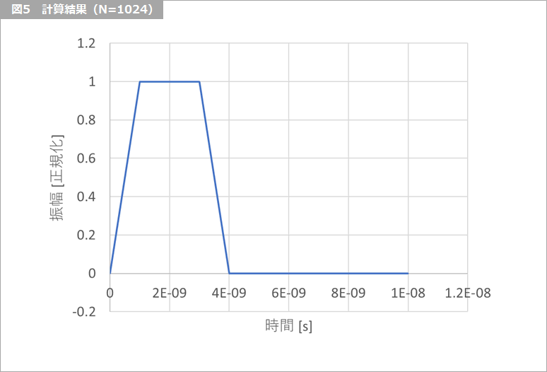
Figure 4 plots time as L2:L65 and amplitude as M2:M65. You can see that the trapezoidal wave in Fig. 1 can be reproduced. This example is an FFT with N=64 for simplicity, and Figure 4 has slight ringing. For a more detailed display, we set N=1024, and we were able to reproduce a clean waveform as shown in Figure 5.

This time, I introduced FFT in Excel. It's a great feature, so please take advantage of it.