- 半導体事業HOME
- マクニカの製品・サービス
-
技術情報

-
イベント・セミナー
- 取扱メーカー
- サポート
- お問い合わせ
- 製品購入はこちら
- 半導体事業のメルマガ登録
![]()
![]() 条件を指定して絞り込む
条件を指定して絞り込む
現在2183件がヒットしています。check
図の番号は前回からの通しです。
縦続行列の活用
ところで、「縦続行列」という名称ですが、これは前回の図1の説明で述べたとおり、縦続接続の解析に適した行列です。
以下のコラムでも少し触れました。
BGAからの配線などで途中でZ0が変わる線路
単に、異なる線路を縦続接続した場合の解析だけでなく、いろいろな場合に活用できます。そのいくつかを紹介します。
容量反射
縦続接続は、線路と線路の縦続接続だけでなく、回路素子との接続にも使えます。
線路と回路素子が接続される場合
回路素子は、入出力間にインピーダンス Z が接続されている場合と、端子間とグラウンド間にアドミタンス Y が接続される基本形を用います。
以下のコラムの図2を参照ください。
縦続行列
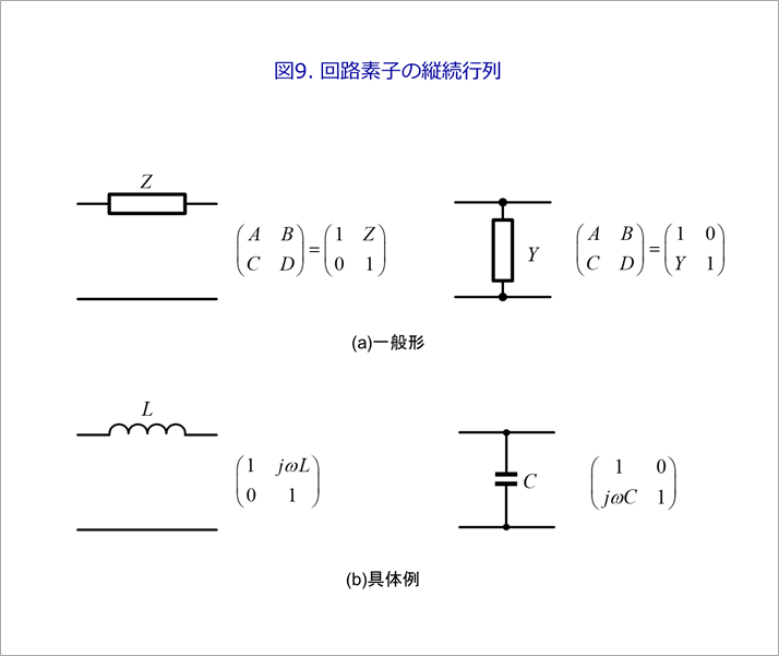
図9(a)に示すように、入出力間にインピーダンスZが接続された場合と、端子間とグラウンド間にアドミタンスYが存在する場合の縦続行列を示します。
同図(b)の具体例に示すように、入出力間のインピーダンスは、インダクタンスLの場合が多く、端子間とグラウンド間のアドミタンスは、キャパシタンスCの場合が多いです。
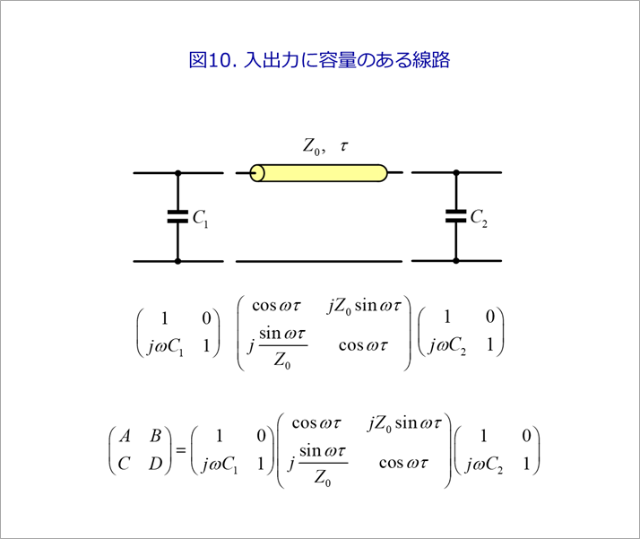
図10のように、近端と遠端にそれぞれ容量C1、C2が接続されます。図9(b)の容量が端子間とグラウンド間にキャパシタCが接続された例を考えます。図10の式は、入力容量C1、出力容量C2を接続した線路の縦続行列です。3つの縦続行列の掛け算は、式を変形するよりも、表計算ソフトを用いる方が格段に容易に求めることができます。
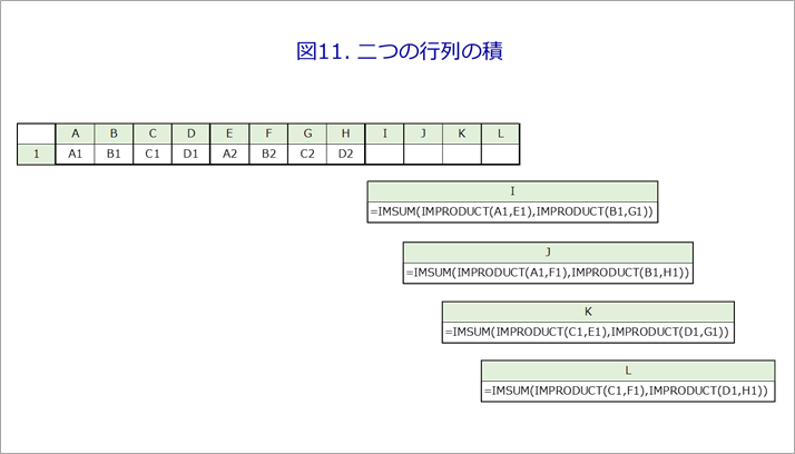
図11は、エクセルによる行列の積の演算です。
第一の行列(A1、B1、C1、D1)をエクセルのセルA1~D1に、第二の行列A2~D2を(E1、F1、G1、H1)に与えます。二つの行列の積をI1、J1、K1、L1に求めます。計算式を同図に示します。複素数演算なので、和はIMSUM、積はIMPRODUCTで求めます。
二つの行列の積を第一の行列とし、新たな一つの行列を第二の行列として、二つの行列の積の演算をコピーすれば、三つの行列の積が求まります。これを繰り返せば、任意の個数の行列の積を求められます。
この結果の縦続行列に対して、図3の式(10)を求めれば、遠端の電圧V2を得ます。これを高速フーリエ逆変換すると時間応答を得ます。
式の展開だけでは面白くないので、実際の計算をやってみます。使用する式は、前回の式(2)と同じく式(10)の二つです。
分布定数回路の遠端の電圧は、式(10)で、縦続行列のA、B、C、Dは、式(2)です。波形の計算は、エクセルによるFFT(その2) に述べたように、筆者の作成した、FFTのエクセルを用います。
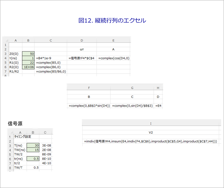
このエクセル(FFT256.xlsx)を用いて、例えば、Sheet1に、図12のように、縦続行列と遠端の電圧を計算します。図12のA列とB列は回路条件で、C4は線路の遅延時間τ(ns)を秒に換算しています。C5からC7は、B5からB7の複素数表現です。D4は、FFT256.xlsxの信号源シートのωとC4のτの積です。E4からH4は、縦続行列です。I4は、前回の式(10)です。信号源は、FFT256.xlsxの信号源のシートの台形波を用いています。
図12の4行を132行まで複写します。FFT256.xlsxの波形のシートのA2に、I4を絶対参照で記入します。Sheet1なら、A2には、「Sheet1!$I$4」と記入します。
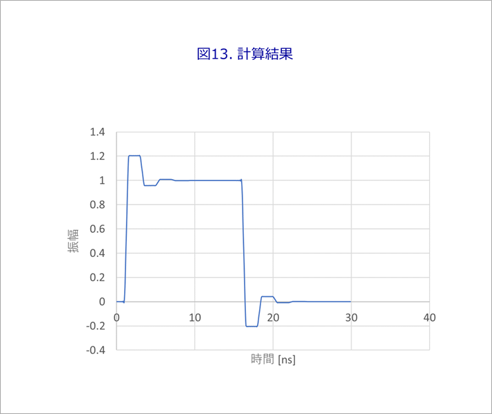
図13が、FFT256.xlsxによる計算結果です。
線路や遠端・近端の条件は、図12の緑色のセル(B3~B6)に任意の値を入力します。信号源の条件は、FFT256.xlsxの信号源のシートの緑色のセル(B3、B4、B6)に任意の値を入力します。
入出力に容量がある場合には、図10の縦続行列に、図11の行列の積を繰り返し用いて得られる縦続行列を用います。
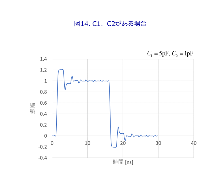
図14に、図10のように、入出力に容量が存在するときの遠端波形を解析して示します。容量の影響を誇張するために、C1=5pF、C2=1pFとしました。
縦続接続の、少し遊びになりますが、分布定数回路のLCの等価回路を、縦続行列の繰り返しで解析してみます。これは、前回の式(2)を用いれば簡単に解析できます。もちろんSPICEを用いても簡単です。あえて「遊び」として解くのは、縦続行列に興味を持っていただきたい思いもあります。
分布定数回路の等価回路は、
分布定数回路~何が分布しているのか?
の図1に示すように、LとCが分布しています。
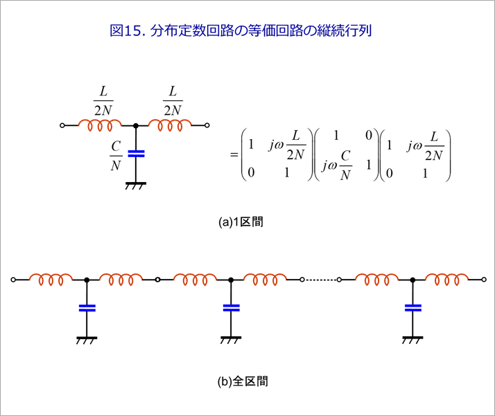
図15は、これを縦続行列に適した書き方です。同図(a)は、全体をN区間に分けたときの1区間とその縦続行列です。同図(b)は、これを全区間つないだものです。(a)の3つの行列の積を1区間として、その2乗を繰り返し演算します。
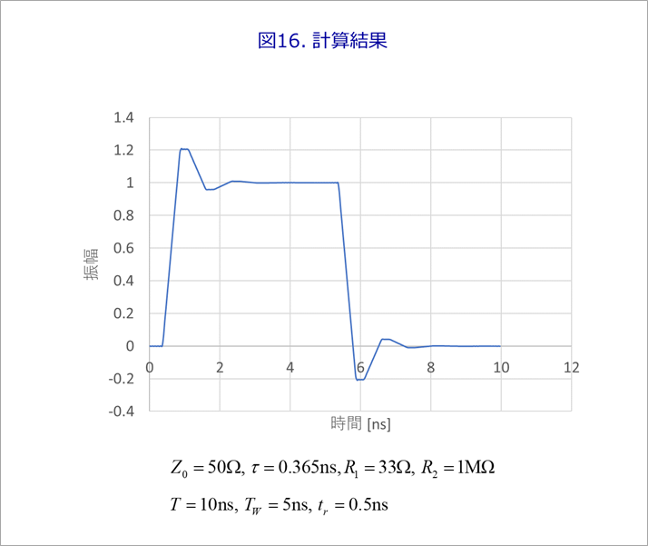
図16は、N=64の場合の反射波形です。図12などと同様に、FFT256.xlsxを用いました。
この例では、N=64で図16のような反射波が得られました。波形を拡大すると、小さな振動が見られます。Nを増やすのは、1区間の2乗の繰り返し演算なので、複写で簡単に行えます。
参考文献
碓井有三 :ボード設計者のための分布定数回路のすべて(第3版)自費出版, pp.146-169, 2016
碓井有三のスペシャリストコラムとは?
基礎の基礎といったレベルから入って、いまさら聞けないようなテーマや初心者向けのテーマ、さらには少し高級なレベルまでを含め、できる限り分かりやすく噛み砕いて述べている連載コラムです。
もしかしたら、他にも気になるテーマがあるかも知れませんよ!