sampling theorem

FFT samples a continuous waveform at discrete times.
The sampling frequency is called sampling frequency.

Modern high-performance oscilloscopes (which have been around for more than 20 years) can sample in real time and display digital data on the screen or capture it as a numerical value.
Such an oscilloscope is called a digital oscilloscope.
An important part of sampling is the sampling theorem (footnote).

It can be completely restored when the maximum frequency component fmax of the target time function f(t) is less than half the sampling frequency fs.
That is, fmax≤fs/2.

Now consider an N=16 FFT with a period T=10ns.
The period of 10ns is sampled at 16 points, so the sampling frequency fs is 1.6GHz and fs/2=0.8GHz.
To satisfy the sampling theorem, the signal frequency must be 0.8 GHz or less.

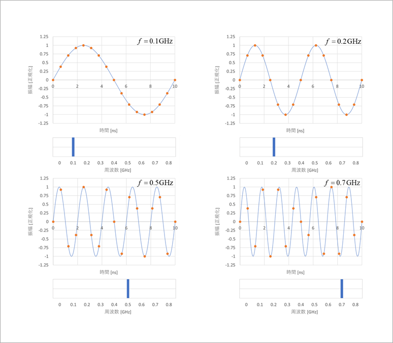
Figure 1 is for f≤fs/2.
Signal waveforms and sampling points indicated by orange markers are shown for signal frequencies of 0.1GHz, 0.2GHz, 0.5GHz, and 0.7GHz.
A Fourier transform of this marker reveals the spectrum of the original frequencies. This is shown at the bottom of the figure.

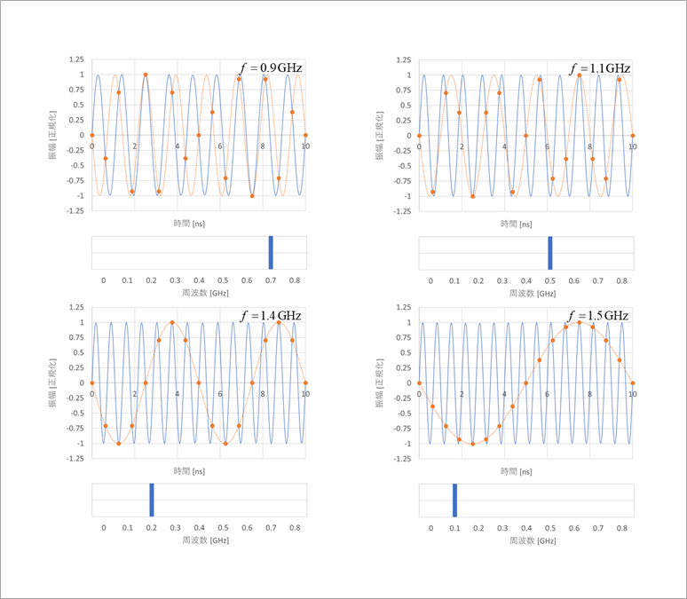
Figure 2 similarly shows the case when the signal frequency f is higher than fs/2.
If the signal frequency is 0.9GHz, a symmetric frequency of 0.7GHz will appear with respect to 0.8GHz at fs/2. However, the polarity sign of the waveform is the opposite (minus) of the original signal.
At 1.1GHz, it is 0.3GHz above 0.8GHz at fs/2, so the frequency that appears is 0.3GHz below 0.8GHz, or 0.5GHz. The same is true for other frequencies in the same figure. This is called folding noise or alias noise because it is folded with respect to fs/2.

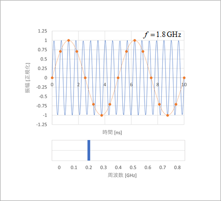
Furthermore, as shown in Figure 3, for 1.8GHz, which is higher than fs(1.6GHz), it folds back with respect to fs. In this case, we wrap about 1.6GHz at fs, so 1.4GHz, which is 0.2GHz wrapping about 0.8GHz at fs/2.
The polarity is the minus of the minus, so it has the same polarity as the original signal.

Therefore, if a signal containing frequency components higher than fs/2 is sampled (digitized) at fs, the high frequency components will be distorted (folded back) into low frequencies, making it impossible to perform faithful waveform conversion.

Alias example

A familiar example is the rotation of the wheels of a western stagecoach that sometimes appears to be reversed.
A movie consists of a sequence of 24 frames of video per second.
In other words, since the sampling frequency is 24Hz, motions above 12Hz, which is half of that, will wrap around at 12Hz.
If a wheel has 12 spokes, the spokes move at 12 Hz when the wheel rotates once per second.
At this time, the wheels appear as if they are standing still, and at higher frequencies, i.e., the stagecoach goes faster, the wheels appear to rotate backwards.
The reason for the reverse rotation can be explained by the fact that the polarity of the sine wave appearing in Fig. 2 is negative.

real example

Consider a real-world example.

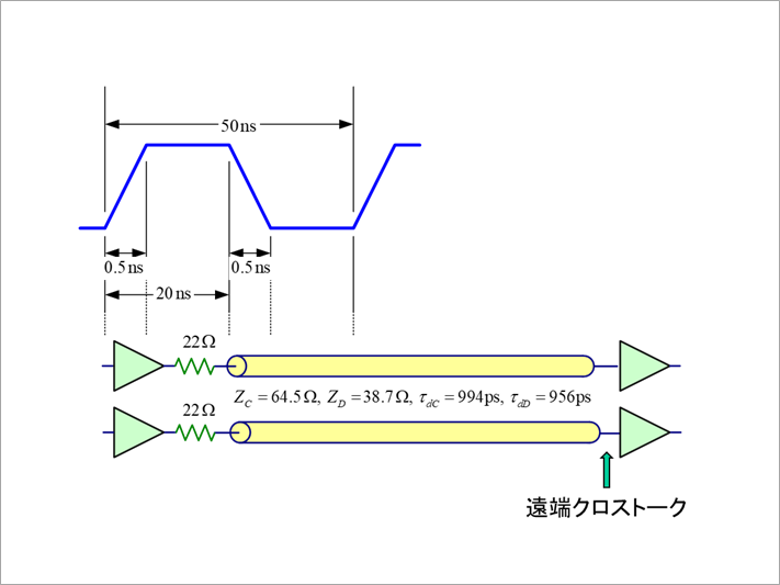
As an example of a waveform with high frequency content, consider the far-end crosstalk waveform of the circuit in Figure 4.
This example assumes a surface layer with a crosstalk coefficient ξ=0.25 and a line length of about 15 cm.

See also

far end crosstalk

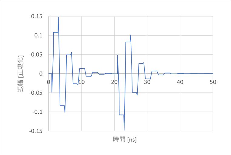
Figure 5 is the analysis result of the far-end crosstalk in Figure 4.
The whisker waveform contains sufficiently high frequency content.
This calculation used FFT with N=16,384 points.

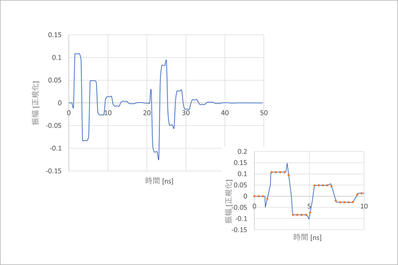
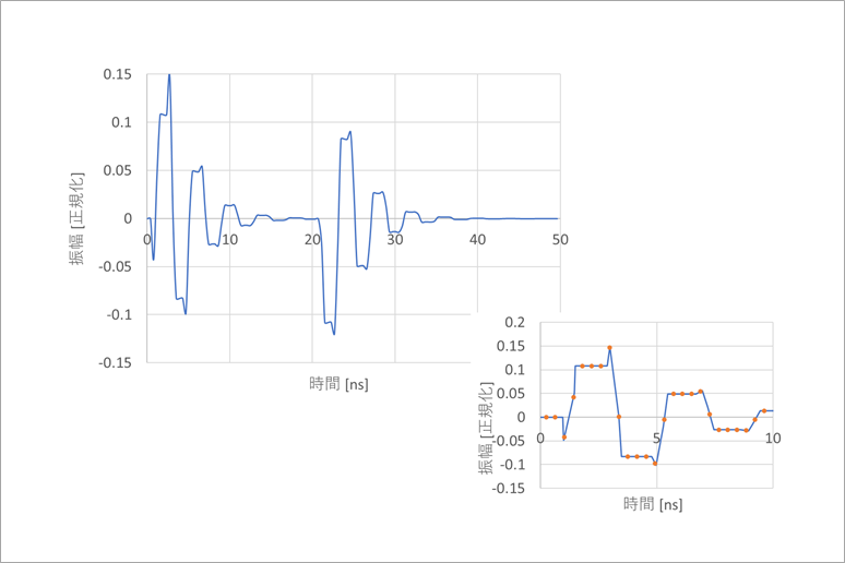
Figure 6 is the inverse Fourier transform (iFFT) of the waveform in Figure 5, sampled at 128 points for one period of 50 ns.
The sampling frequency fs is 2.56GHz (1/50ns x 128).
Fig. 6(a) is sampled outside the first whisker-like peak, and Fig. 6(b) is sampled just over the peak.
It turns out that the 128-point FFT is not a good fit, as the sampling points may or may not coincide with the peak points of the waveform.

The reason for this is that the waveform in Figure 5 contains frequency components above half the sampling frequency.

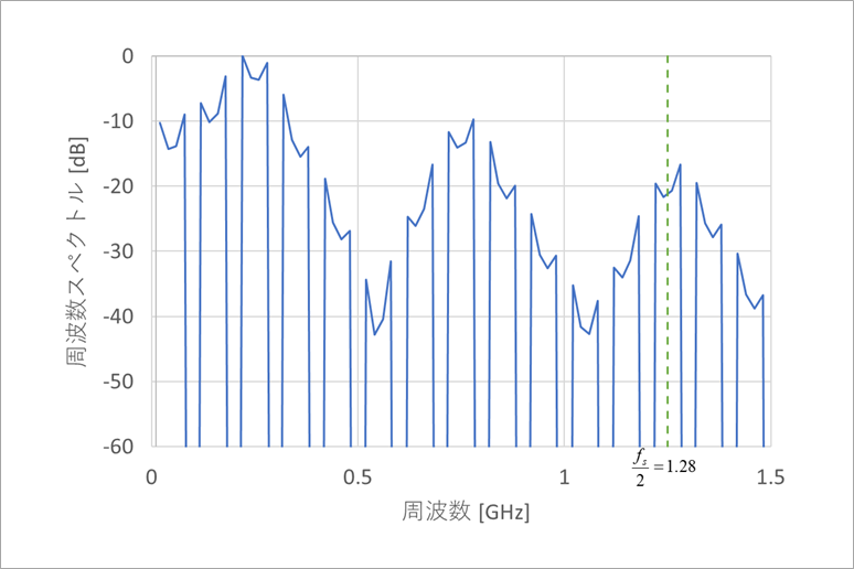
Figure 7 is the frequency spectrum of the waveform in Figure 5.
Normally, frequency characteristics are represented by a logarithm on the horizontal axis (frequency), but here a linear memory is used to represent folding.
Sufficient spectrum is present at frequencies above 1.25GHz at fs/2.

To suppress this high frequency component, a low-pass filter (LPF: Low Pass Filter) is usually used.
This filter is called an anti-alias filter in the sense that it removes aliases.

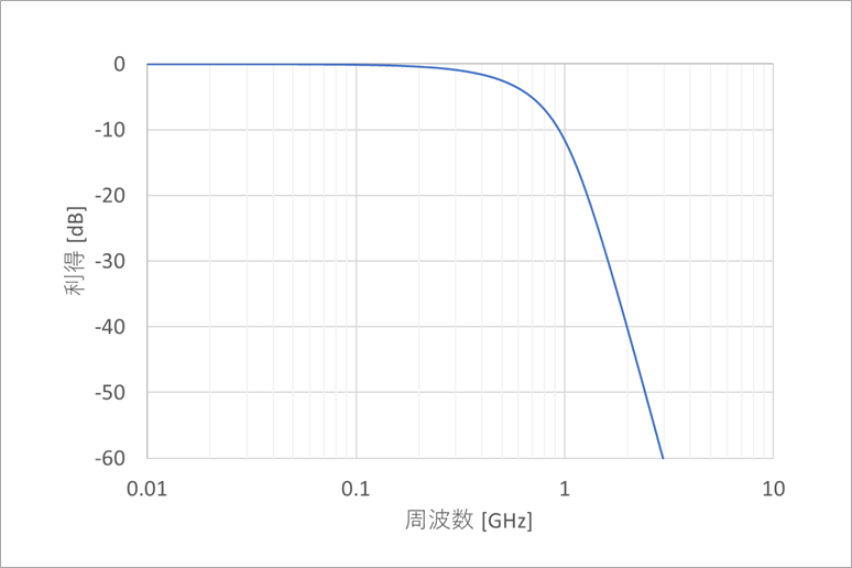
Figure 8 is an example of an LPF with 20dB attenuation at fs/2 (1.28GHz).
There are various types of filters, but the Bessel type is used for pulse waveforms.
The figure is a 6th-order Bessel filter.
The characteristic of Bessel filters is that the attenuation characteristics are gentle, but the group delay is constant, so the waveform distortion can be kept small.
I will discuss the filter characteristics on another occasion.

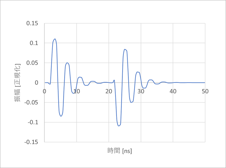
Figure 9 is the 128-point inverse Fourier transform of the original waveform (Figure 5) with the anti-aliasing filter of Figure 8 applied.
Of course, even if the sampling point shifts, the waveform will not change.

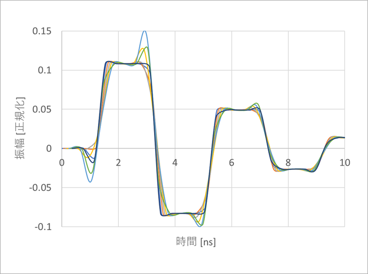
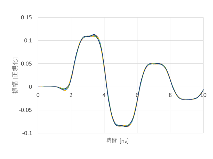
Figure 10(a) shows the superimposed waveforms when the sampling points in Figure 6 are changed.
It can be seen that the waveform differs greatly depending on the variation of the sampling point.
The same figure (b) shows the case when an anti-aliasing filter is added.
The same waveform can be obtained even if the sampling point fluctuates.
The rise point of (b) in the same figure is shifted by a little less than 1 ns compared to (a). This is the delay due to inserting the anti-aliasing filter.

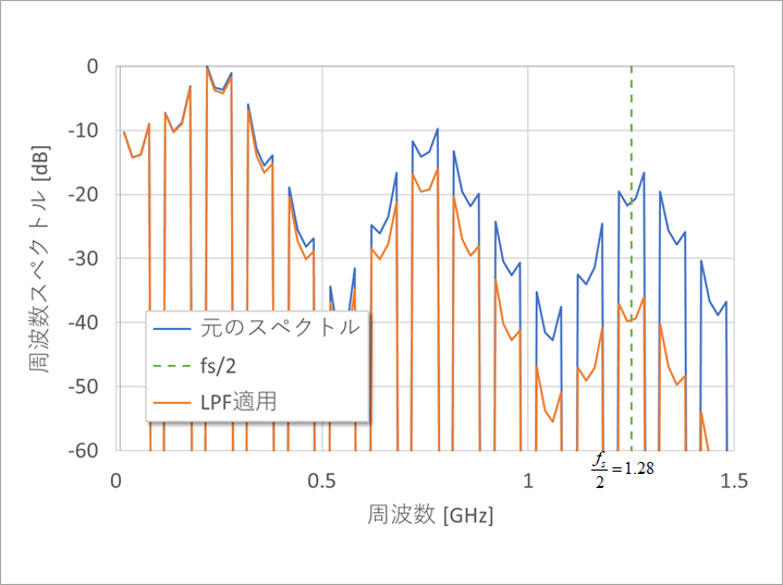
Figure 11 shows the change in spectrum due to the application of LPF. It can be seen that there is sufficient attenuation at frequencies higher than fs/2.

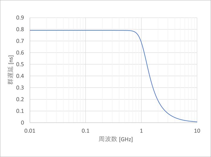
Figure 12 is the group delay of the LPF in Figure 8. A feature of the Bessel filter is that it is flat up to around 1 GHz.
If there is an opportunity, I would like to describe this delay characteristic in comparison with other filter types.

footnote

This is called Shannon's sampling theorem.
It is called the Nyquist-Shannon theorem because Nyquist first conjectured it, and it is also called the Someya-Shannon sampling theorem because Japanese Isao Someya announced it at about the same time as Shannon.

bonus

At the stagecoach, I mentioned that the film has 24 frames per second.
Modern televisions are at 30 frames per second.
Movies don't play well on TV. Conversion from 24 frames to 30 frames is required.
How is this conversion done?
If there is an opportunity, I would like to write it in the trivia corner.
When I was a boy (did you go to junior high school?), I asked NHK, and they kindly wrote several sheets of report paper explaining how to do this conversion and sent it to me.