Equivalent circuit and equation

As with reflection, consider the equivalent circuit of Figure 1.
Mutual inductance LM between lines and capacitance CM between lines are newly added compared to a single line.

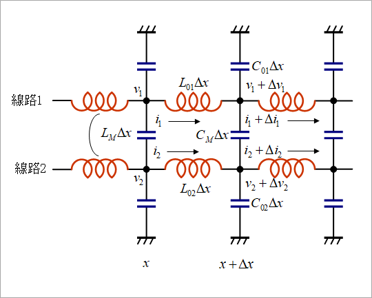
Including the coupling term, set up the equation for line 1 as shown in the upper left of Fig. 2.
Since the voltage and current equations are not symmetrical, put C01+CM=C1 and CM=-Cm as shown by the arrows in the middle of Fig. 2, and transform them as shown on the right side of the figure. The voltage formula can be left as it is, but in order to make it easier to see together with the current formula, simply replace it with L01=L1 and LM=Lm.

Similarly, formulate the equation for line 2, and obtain a partial differential equation in the same way as for reflection.
Note that this transformation of the formula is not required. I see many examples of solving without transforming, but I think it is easier to transform.
Represent the voltage and current equations in matrices.

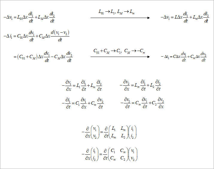
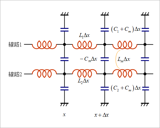
Figure 3 is an equivalent circuit corresponding to the modified expression. Note that Cm is negative here. Coupling capacitance is often displayed as a minus value in software that calculates line constants. Understand that the negative meaning comes from the transformation of the formula.

Find the voltage from the system of equations

As in the case of reflection, the partial differential equation is Laplace transformed into an ordinary differential equation, as shown in Figure 4.
Differentiate the voltage equation twice and substitute the current equation into the voltage-only equation.
Differentiating the second derivative of V1 of the voltage equation twice more and substituting the second derivative of V2 into the equation for the fourth derivative of V1 yields the fourth differential equation with respect to V1.

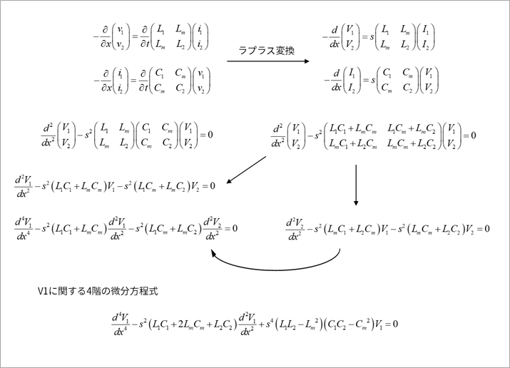
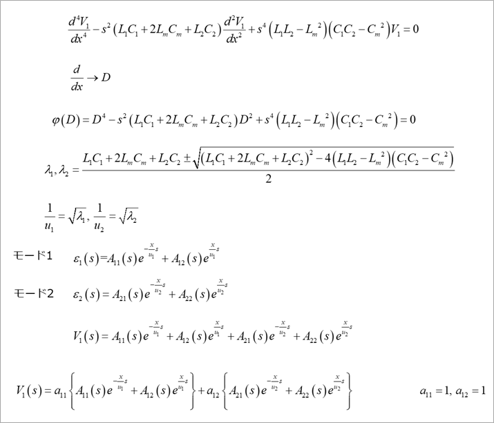
Let d/dx of this 4th-order differential equation be the differential operator D. (symbolic solution)
φ(D) is a biquadratic equation, and the square of the root of φ(D)=0 (D^2) is defined as λ1 and λ2. I want it.
Let V1 be the sum of two waves ε1 and ε2 of modes 1 and 2 (the simplest form of first-order coupling). For symmetrical circuits, these are common and differential modes.
where the square root of λ is the delay time of each wave and is the reciprocal of the velocity u.
The first term on the right hand side of ε1 in mode 1 is the right-going wave (the wave traveling to the right) and the second term is the left-going wave. The coefficients A11 and A12 are the constants of integration and will be determined later by the boundary conditions.
Express the V1 equation as a linear combination of Mode 1 and Mode 2 by multiplying the coefficients of a11 and a12 (here, both are 1).

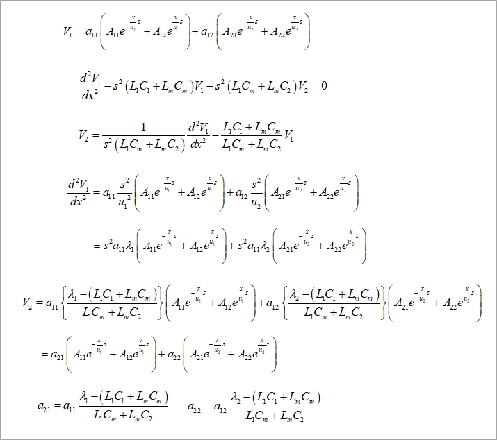
Obtain V2 as shown in Figure 6 from the second derivative formula of V1 in Figure 4.
V2 can be obtained by substituting the final V1 formula in Fig. 5 and the second derivative of V1 into this formula.
This expression is also a linear combination of ε1 and ε2. Let the respective coefficients be a21 and a22 as shown in the figure.

find the current

Solve the current from the voltage equation as shown in Figure 7.
Find the current from the voltage equation in Figure 4. Find the derivative of the voltage in this equation.
Substituting this differential equation into the current equation obtained above, we obtain I1 and I2.
Current, like voltage, is expressed as a linear combination of modes 1 and 2. The letter on the left side of these equations is the Greek letter ι (iota).

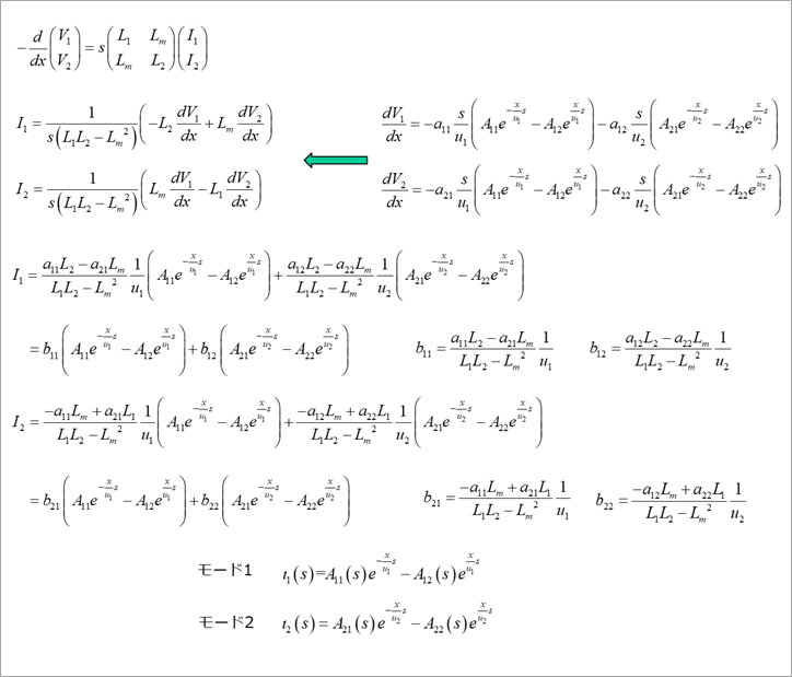
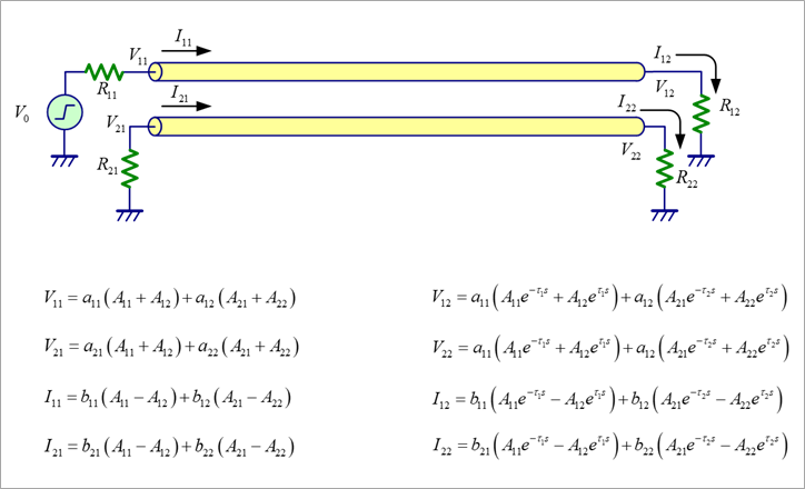
If the near-end and far-end voltages and currents are determined for the circuit in Figure 8, the relationship between voltage and current is shown in the figure.

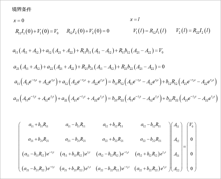
Find the Constant of Integration by Boundary Conditions

Figure 9 shows the near-end and far-end boundary conditions. Substituting the voltage and current equations in Figure 8 into these four equations yields a system of equations for the four constants of integration, A11, A12, A21, and A22.

Solving the simultaneous equations for A11-A22 and substituting them into the equations in Figure 8 gives the near-end and far-end voltages.
For now, let's just set up the system of equations.

It's a four-element simultaneous equation, so it's not so easy, but you can get the time function by inverse Laplace transform of the solution.
Please refer to my book about symmetrical lines.

Next time, I will discuss some solutions.