- 半導体事業HOME
- マクニカの製品・サービス
-
技術情報

-
イベント・セミナー
- 取扱メーカー
- サポート
- お問い合わせ
- 製品購入はこちら
- 半導体事業のメルマガ登録
![]()
![]() 条件を指定して絞り込む
条件を指定して絞り込む
現在2183件がヒットしています。check

ラプラス変換とフーリエ変換については、以前、以下に述べました。
ラプラス変換とフーリエ変換
ラプラス変換とフーリエ変換 その2
「ラプラス変換とフーリエ変換 その2」では、信号源を折れ線としました。
その結果、曲がり角の高い周波数成分を、FFTでは忠実に再現できないため、この回で予告したように、滑らかな波形での比較が必要です。
滑らかな信号源として、矩形波形をベッセルフィルターを通した波形を用います。
ベッセルフィルターについては、以下を参照ください。
ベッセルフィルターと他のフィルターの違い その1
ベッセルフィルターと他のフィルターの違い その2
以前にも述べたように、ラプラス変換は過渡現象で、フーリエ変換は周期関数なので、厳密に比較するには、以下の二つの方法をとる必要があります。
(1)フーリエ変換を孤立波に近似する
(2)ラプラス変換を疑似周期化する
(1)は、信号のデューティー比を小さく選びます。同じパルス幅の解析でも、デューティー比が半分(周期が2倍)になると、フーリエ変換の有効なNが半分になる、逆にいうと、同じ解析精度を得るためには、2倍のNが必要になります。
(2)に関しては、図1で説明します。
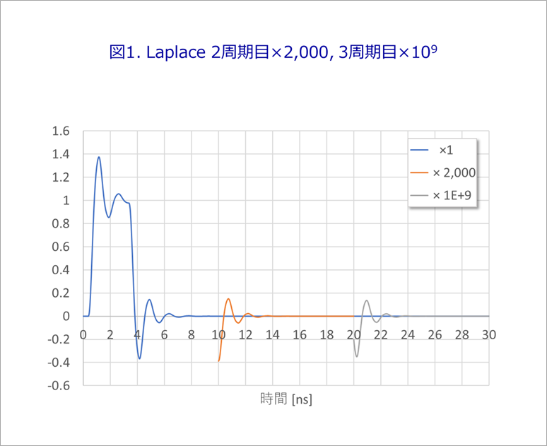
ここでは、比較するフーリエ変換の周期 T を10nsとします。
図1の青線はラプラス変換した、パルス幅3nsの単発の反射波形です。
図では、数nsで波形の振動(反射)は落ち着いているように見えますが、例えば、10ns付近を 2,000 倍に拡大(橙色の線)すると、反射の残骸を確認できます。
さらに、20ns付近を10の9乗に拡大(灰色の線)すると、まだ反射は完全には落ち着いていません。
したがって、ラプラス変換を疑似周期化するには、図1の10ns以降と、20ns以降の反射の残骸を元のパルス波形に加算する必要があります。
なお、(1)および(2)は、ラプラス変換とフーリエ変換を厳密に比較するために用いる手法で、実用的には、全く必要ありません。
図2(a)に、単発波形とフーリエ逆変換したものの差を示します。
ブルーの線が差(左軸目盛)で最大で200ppm程度の誤差があります。灰色の線(右軸目盛)は、信号です。
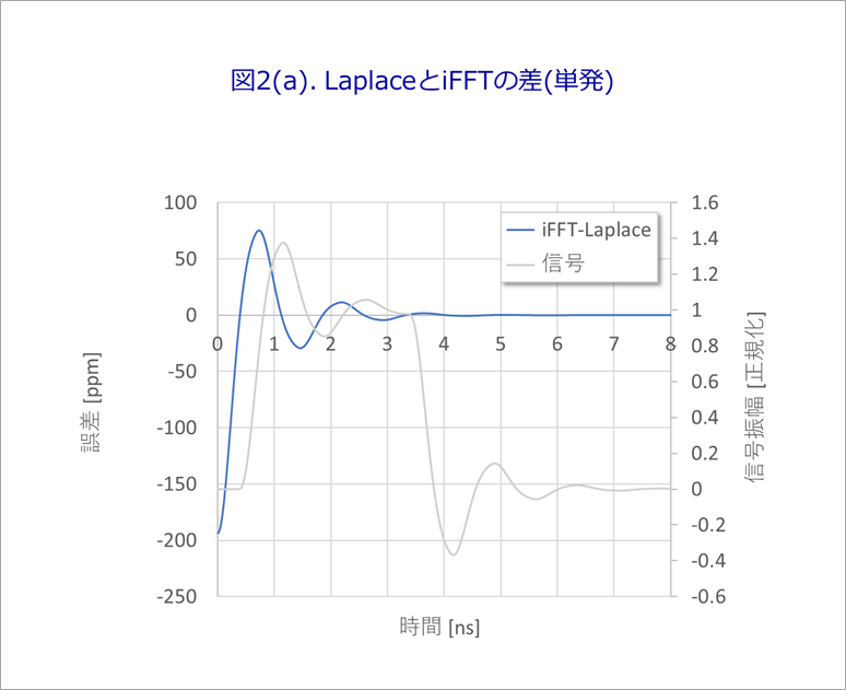
その原因は、図1の10ns付近のオレンジの波形や20ns付近の灰色の波形の重なりに起因します。
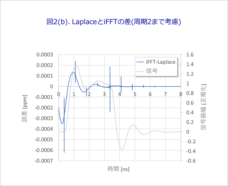
図2(b)は、ラプラス変換に、オレンジの波形を重畳して、フーリエ変換と比較したものです。
誤差の最大値もピークで0.0006ppmと、ほぼゼロになりました。
さらに、図1のグレーの波形まで重畳すると、図2(c)のように、針状の誤差のみとなりました。
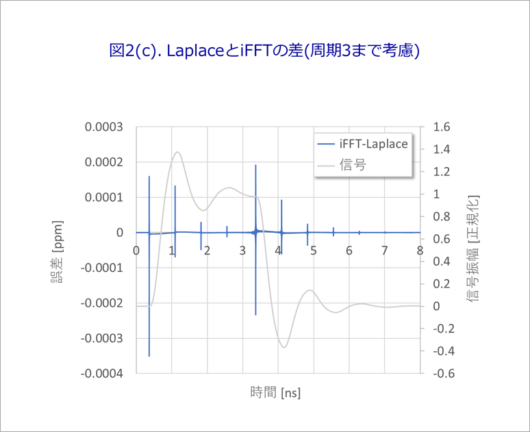
図3に、「ラプラス変換とフーリエ変換2」の図4に、信号波形を重ねて書き直しました。
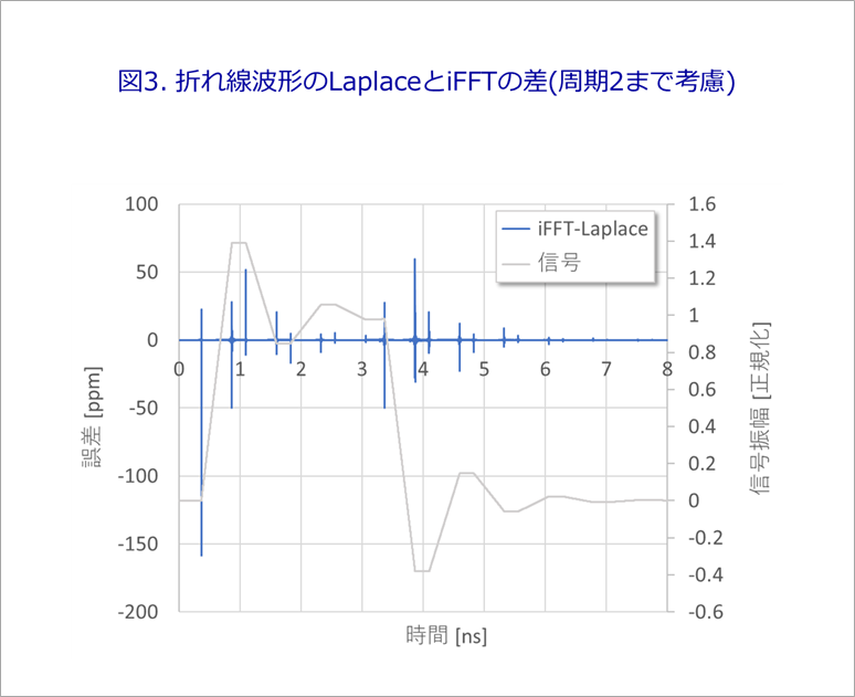
折れ線の信号の場合には、変化時に誤差が大きくなり、最大で150ppm程度の誤差となります。
図2(c)と図3とを比べると、5桁以上の違いがあります。
以上の図は、いずれもiFFTのNは、16,384です。
次に、iFFTのNと解析誤差について検証します。
まず、折れ線の信号の場合の誤差です。
図4は、iFFTのN=256とN=512の場合の誤差です。3,000ppmから4,000ppm、すなわち、0.3%から0.4%程度の誤差です。
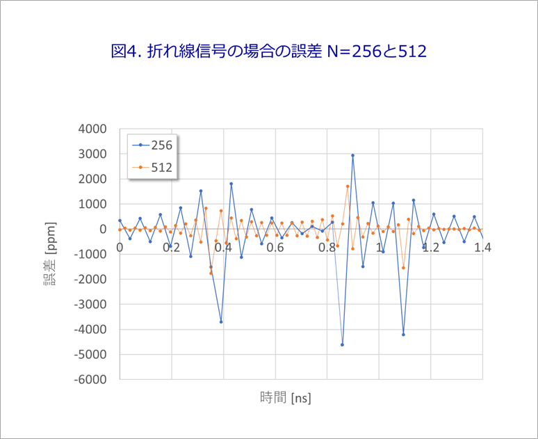
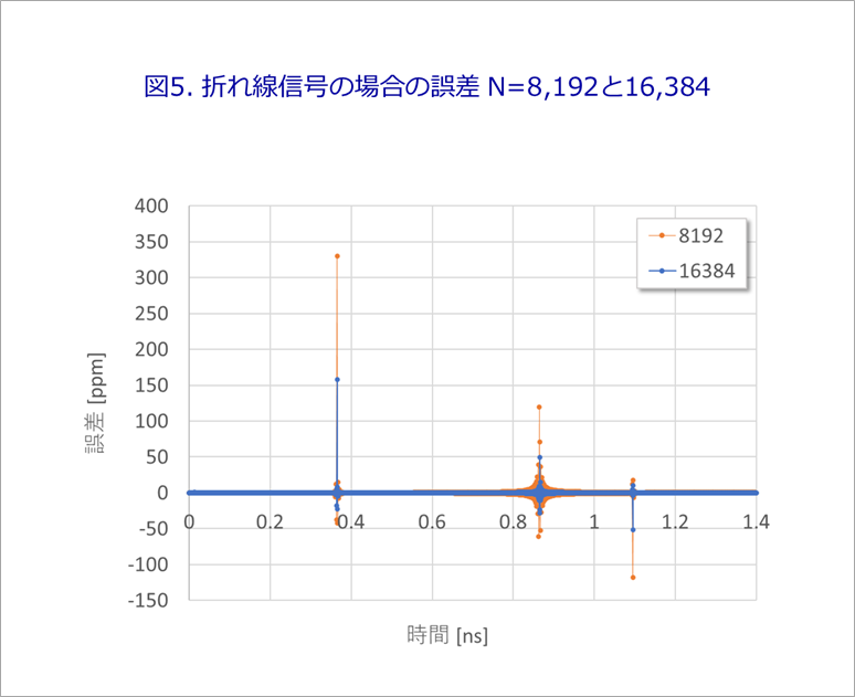
図5は、N=8,192とN=16,384の場合の誤差です。平坦部は小さい誤差ですが、前に述べたように、波形の曲がり角で誤差が生じています。
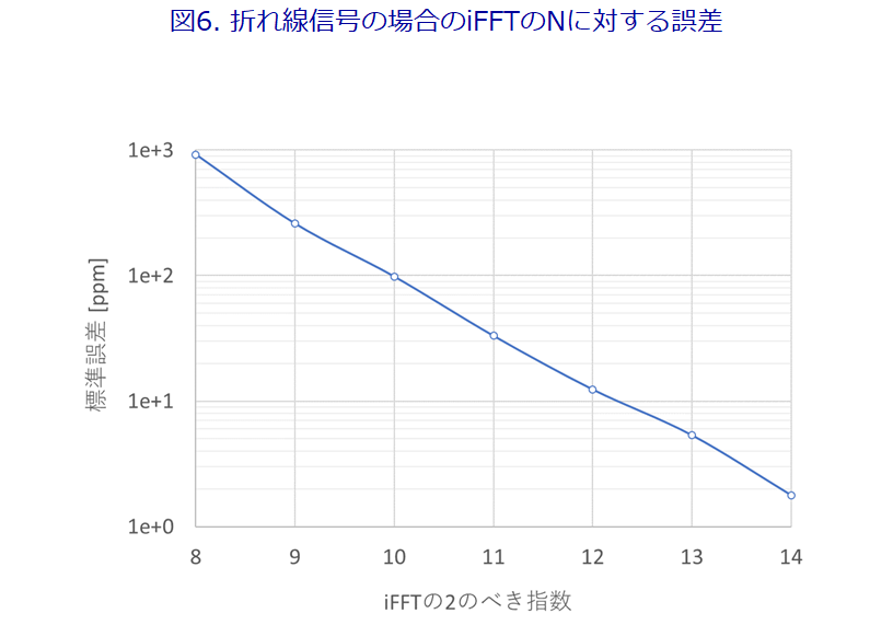
誤差を検証するために、各時間のタイミングの誤差の標準誤差=二乗平均平方根(RMS : Root Mean Square)を計算します。
図6は、折れ線信号の場合のiFFTのNに対する誤差です。横軸は、FFTの2のべき指数で、例えば、横軸が10の場合は、Nは2の10乗、すなわち、1,024です。
N=16,384(2の14乗)で、標準誤差が2ppm程度です。
次に、今回の、ベッセルLPFを用いた滑らかな信号の場合について検証します。
図7は、N=256と512の場合のベッセルLPFの場合の誤差です。折れ線の図4と比べてください。
N=256の場合に、ピークで60ppm程度の誤差で、N=512の場合は、ピークでも10ppm以下です。
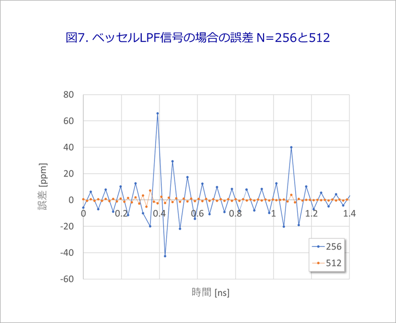
図8は、N=8,192と16,384の場合のベッセルLPFの場合の誤差です。折れ線の図5と比べてください。
いずれの場合も、極めて小さな誤差です。
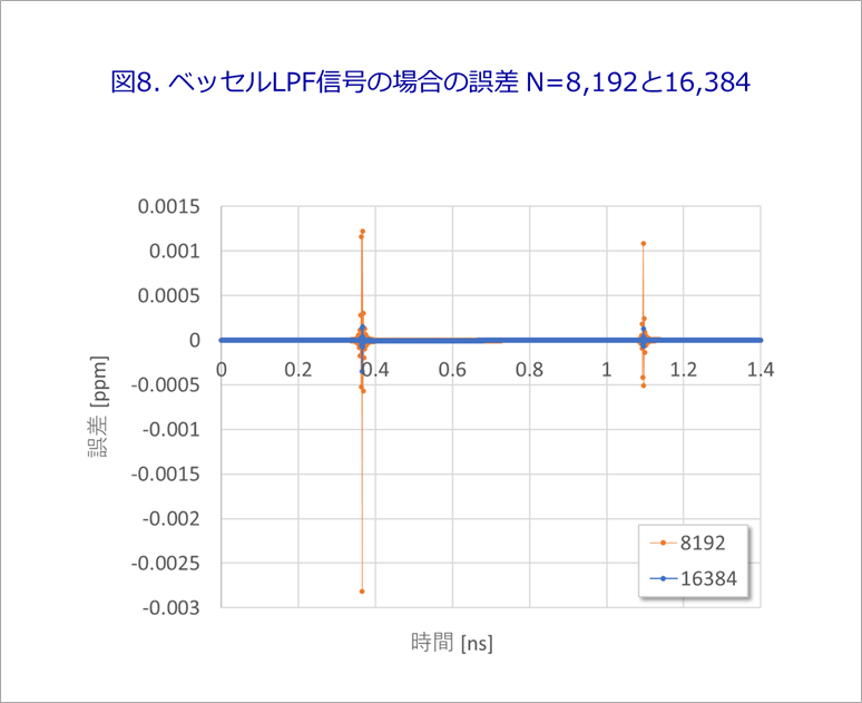
図9は、折れ線の図6に対応した、ベッセルLPFの場合の標準誤差です。
N=256(2の8乗)で10ppm程度です。
2のべき指数の増加に対応して、1桁以上誤差が小さくなります。
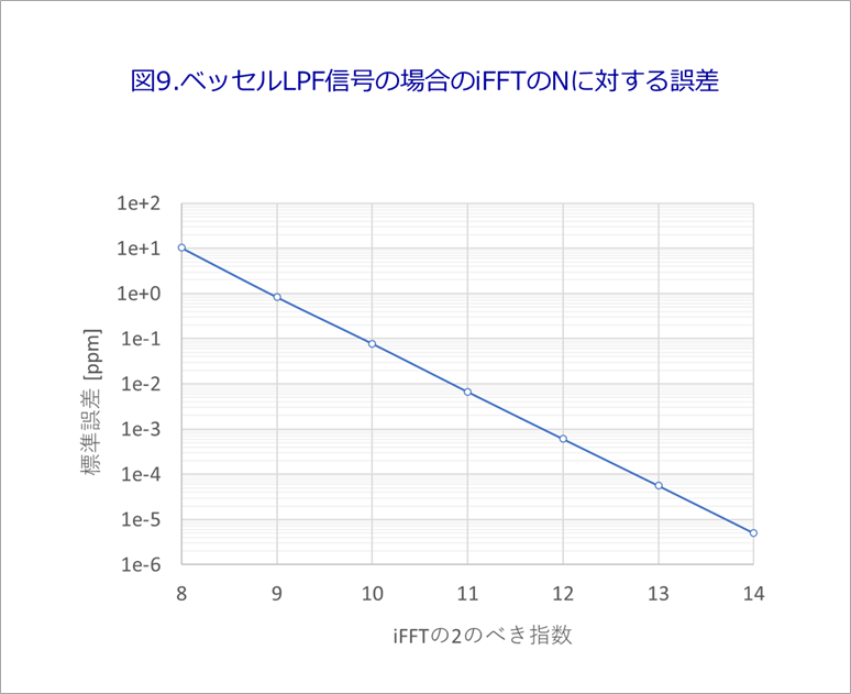
実用的には、N=256でも十分な精度(誤差)と考えます。
図10は、折れ線の場合のiFFT(N=256)とLaplaceの波形の比較です。
iFFTは、最初の立ち上がり後の平坦部に、ジグザグのうねりが見られます。
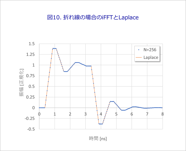
両者の誤差は、図7のプルーの波形です。
0.4ns付近で、60ppm程度の誤差があります。
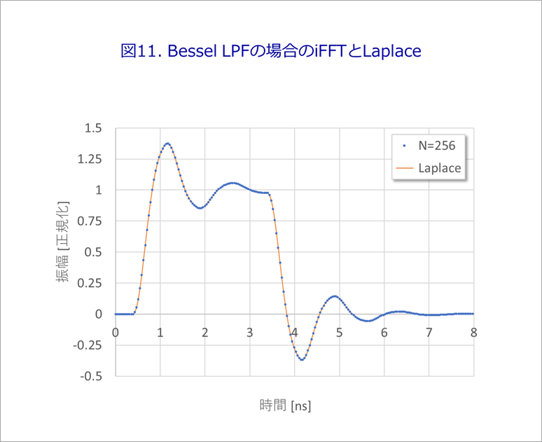
図11は、矩形波をBessel LPFに通した場合の、iFFT(N=256)とLaplaceの波形の比較です。
目で見る限りは両者の波形のズレ(誤差)は認められません。
フーリエ変換のNをどのように選ぶかは、解析する波形の高周波成分によっても異なりますが、通常の反射波形の場合、折れ線の波形なら、1,024と考えます。
この場合、標準誤差は100ppm程度です。図6を参照ください。
折れ線ではなくて、ベッセルLPFで生成した波形の場合、図9によると、N=256でも標準誤差は10ppmなので、十分と考えます。
フーリエ変換とベッセルLPFについては、数回に分けて述べました。
幸いなことに、PCの性能が向上して、N=4,096程度の高次のiFFTでも性能上の問題は感じられません。
是非活用していただければと思います。
なお、筆者の環境(Core i5-12600KF)では、N=16,384程度が限界と感じました。
碓井有三のスペシャリストコラムとは?
基礎の基礎といったレベルから入って、いまさら聞けないようなテーマや初心者向けのテーマ、さらには少し高級なレベルまでを含め、できる限り分かりやすく噛み砕いて述べている連載コラムです。
もしかしたら、他にも気になるテーマがあるかも知れませんよ!