What is Monte Carlo Analysis?

Monte Carlo analysis uses random numbers to generate random combinations of component tolerances, making it possible to check changes in circuit behavior.
This allows you to predict circuit yield and verify component values that meet design specifications.

Let's use the mc function to see the variation in resistance

Monte Carlo analysis in SPICE generally gives pseudo-random numbers (functions) as part errors and fluctuates parameters.

LTspice does not have a menu for automatic Monte Carlo analysis, so use a combination of function specification and the Step command.

This time, I would like to use the mc function.
The mc(x, y) function generates uniformly distributed random numbers between x*(1+y) and x*(1-y) values.

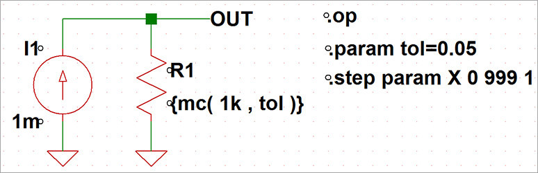
First, assign a function to the resistance value as shown in Figure 1.

In this example, set a resistance of 1kΩ (5% nominal error) with {mc( 1k, tol )}.
Next, use the Step command to repeat 1000 times from 0 to 999.

The simulation results are shown in Figure 2.

This time, the variation in the voltage generated across the resistor is confirmed as the variation in the resistance.
The vertical axis is the voltage value generated in the resistance, and the horizontal axis is the number of steps.

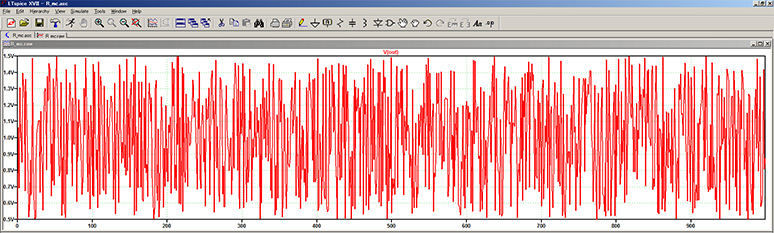
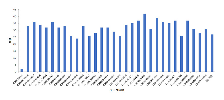
Figure 3 is a histogram of this graph data imported into Excel.
It can be seen that the voltage (resistance) variation generated in the resistor has a uniform distribution.

Consider the cutoff frequency of the filter

The nice thing about Monte Carlo analysis is that you can see how multiple component parameters relate to each other.
Here, we will make an RC filter using two parts, a resistor and a capacitor, and check the variation of the cutoff frequency.

The resistor used is 1k±0.5%(ohm) and the capacitor is 0.01u±20%(F). , 0.1)}.

The number of repetitions is a total of 1000 times from 0 to 999 using the Step command.

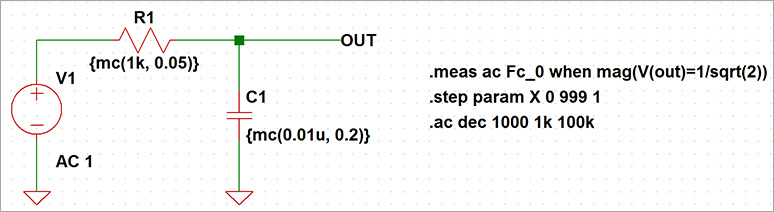
The simulation result (AC characteristics) is shown in Fig. 5, and the -3dB point on the gain (vertical axis) is the cutoff frequency.

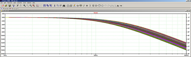
In Fig. 5, the results are difficult to understand, so I calculated the cutoff frequency (-3db) points with the ".meas" command and summarized the resulting dispersion in a histogram (Fig. 6) in Excel.

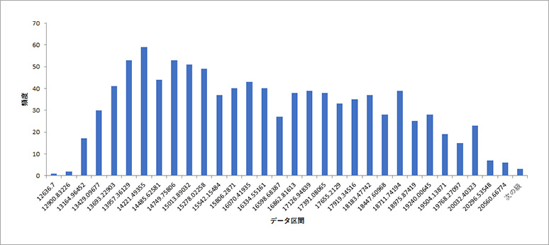
The cutoff frequency without error is Fc = 1/(2*π*R*C) = 15.915kHz (about 16kHz).
This time, we added a uniformly distributed random number and multiplied the resistor and capacitor, so it should look like a normal distribution of the minimum value (approximately 12.6kHz) and maximum value (approximately 20.6kHz) of the cutoff frequency. . However, this time, there is a difference in the variation between resistors and capacitors, and the capacitor has a large error of 20%.

If you download the demo file and create a histogram distribution with the same 5% error, you will get a normal distribution.

Please download it and check it out.

LTspice demo file verified this time

After extracting the zip file to the same folder on a computer with LTspice installed, run LTspice to automatically start waveform display.

R_mc__1.zip

Uniform distribution of resistance R_simulation file

RC_mc__1.zip

Uniform distribution of RC circuit_simulation file

At the end

This time, I introduced an example of Monte Carlo analysis in LTspice.

By setting the variation and simulating it, you can understand the behavior of the circuit and the degree of influence on the entire system. However, it is necessary to consider separately whether the function to be given should be a uniform distribution or another random number function should be used.

LTspice supports various functions (Gaussian, etc.), so please try them if you have the chance. These functions can be found in LTspice's Help menu.

We also hold regular LTspice seminars. You can learn the basic operation of LTspice, so please join us.

Click here for LTspice seminar information

Inquiry

If you have any questions regarding this article, please contact us below.