Eigen equations and eigenvalues

Start from the Laplace transform formula in the upper right of Fig. 4 in Part 1.

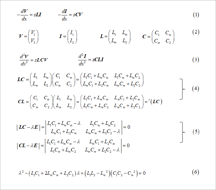
Here, we use vector notation as shown in formula (1) in Figure 1. The vector of each variable and coefficient is shown in equation (2). Note that vectors are shown in bold. Differentiate the voltage equation of equation (1) with respect to x and substitute the current equation. Similarly, differentiate the current equation and substitute the voltage equation to obtain the second-order differential equation of equation (3) get LC and CL are calculated and shown in equation (4). LC and CL are the transposed matrices of each other.

A transposed matrix is a matrix whose rows and columns are interchanged. Here, the notation is superscripted with a t in front of the symbol. The two propagation velocities u1 and u2 were obtained by symbolically solving the fourth-order differential equation using the symbol D, as shown in Fig. 5 of Part 1. λ in the figure can be found by solving the equation (proper equation) for λ in equation (5) in Fig. 1. where E is the identity matrix.

Equation (5) is a quadratic equation with respect to λ, so λ can be obtained from the root formula. Formula (5) is expanded to formula (6). The roots λ1 and λ2 of this equation are called eigenvalues.
As is clear from equation (5), voltage and current have the same eigenvalue.

Eigenvector

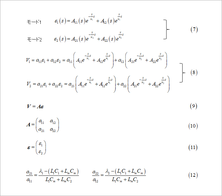
Equation (7) in Figure 2 describes a two-mode wave propagating in this coupled line. We will name these ε1 and ε2. For symmetrical lines, these two modes correspond to the common and differential modes.
Each of ε1 and ε2 is represented by the sum of right and left waves (first-order coupling).

A11 to A22 are the integral constants of the differential equation determined from the boundary conditions at the near and far ends. Equation (8) means that the voltage on the two lines is represented by the linear combination of the two mode waves. Equation (9) is the vector representation of Equation (8). A and ε in vector notation are Eqs. (10) and (11). The linear coupling coefficients a11 to a22 in Equation (8) represent the line with the first number in the coefficient suffix and the mode with the second number. In part 1, we set a11=a12=1, but as shown in equation (12), it is expressed by the ratio of line #1 and line #2 in each mode.

This ratio is called an eigenvector.

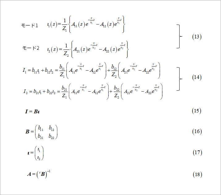
Similar to voltage equations, currents are summarized in Figure 3. Corresponding to equation (7), the two modes of current are shown in equation (13). The voltage is the sum of the right and left waves, but the current has a direction, so it is the difference between the two. Divide the difference in braces by the characteristic impedance of each mode to get the current for each mode. Corresponding to equation (8), the current is also represented by the linear combination of the two modes.

Equation (15), like Equation (9), is the vector notation of Equation (14). In vector notation, B and ι (the Greek letter iota) are Eqs. (16) and (17). In the equation for current, Figure 1, equation (3), the coefficient CL for current I is the transposed matrix of LC for the voltage equation. See equation (4) in Figure 1. Since the eigenvalues of LC and CL are equal, the relationship between matrix A consisting of two eigenvectors of LC and matrix B consisting of two eigenvectors of CL is given by Equation (18).

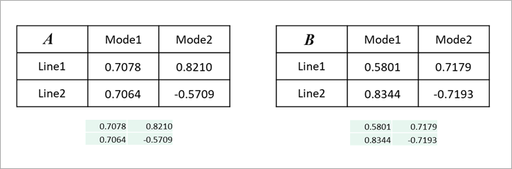
The eigenvectors were obtained by the calculation in Fig. 6 in Part 1, but in a smarter way, the eigenvalues λ1 and λ2 are obtained as x1 and x2 in equation (19) in Fig. 4, respectively. Eigenvectors are normalized for each mode as shown in Equation (20).

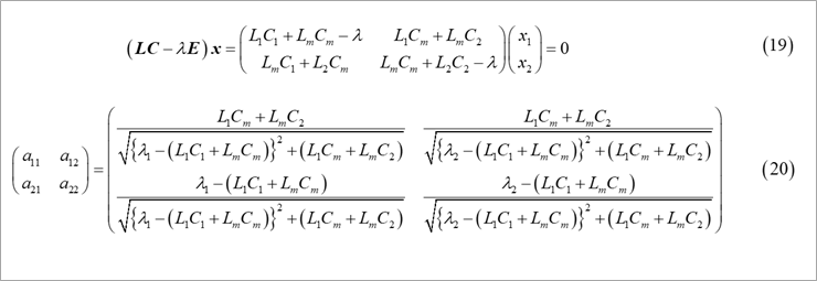
Table 1 shows an example of actual calculations for the example in Figure 5 of Part 2.

Propagation constant for each mode

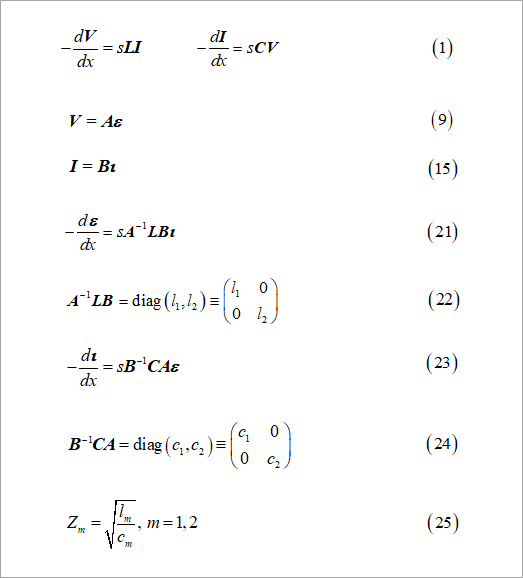
Some of the equations needed to find the propagation constant for each mode are reproduced in Figure 5.

Equation (1) is the basic equation for voltage and current. Equations (9) and (15) are the relationship between the voltage and current, and the voltage and current of each mode.
From equations (1) and (9), the relationship between voltage and current in each mode is given by equation (21).
Comparing the voltage formula of formula (1) with formula (21), the coefficient of ι is the inductance l1 (L1) and l2 (L2) of each mode as shown in formula (22). increase.
Similarly, from Equations (1) and (15), the relationship between current and voltage in each mode is given by Equation (23), and the coefficient of ε is the capacitance c1 and c2.
From the inductance and capacitance obtained from equations (22) and (24), find the characteristic impedance of each mode as shown in equation (25).

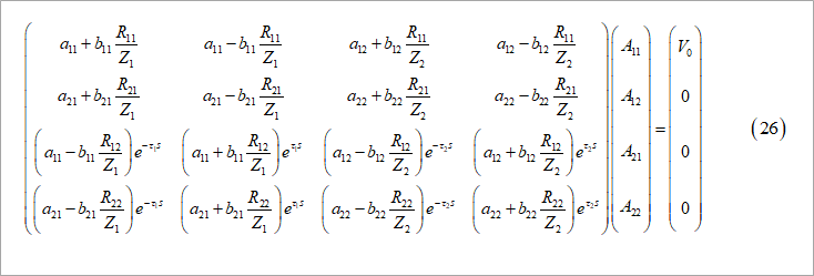
Similar to Figure 9 of Part 1, we give the boundary conditions and obtain the equation in Figure 6, Eq. (26).
Obtain each coefficient in turn and calculate the near-end and far-end waveforms by Laplace transform or Fourier transform.
Note that the same symbols (a11 and b11) as the coefficients 1 and 2 are used, but of course the values are different.

References

Yuzo Usui: All About Distributed Constant Circuits for Board Designers (3rd Edition) Self-published, 2016
CRPaul: Analysis of Multiconductor Transmission Lines, 2E, Wiley-IEEE Press, 2007
What is Yuzo Usui's Specialist Column?
It is a series of columns that start from the basics, include themes that you can't hear anymore, themes for beginners, and also a slightly advanced level, all will be described in as easy-to-understand terms as possible.
Maybe there are other themes that interest you!