distribution constant

The fact that capacitors and inductors are distributed on the line is known as "Distributed constant circuit - what is distributed?’ said. In order to describe crosstalk quantitatively, it is necessary to understand the lines that are coupled together, that is, the capacitors and inductors of the coupled lines.

negative capacitance

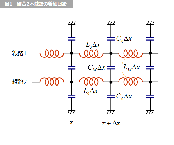
In the case of two tracks, in addition to the parameters of the track itself, there are parameters between the tracks as shown in Fig.1. CM is the line-to-line capacitance and LM is the mutual inductance.

The voltage and current of this equivalent circuit are expressed by equations (1) and (2) in Fig. 2, but the symmetry of each equation is not good, so if the capacitor is replaced by equation (3), The formula has good symmetry. Incidentally, the inductor is also replaced according to the capacitor as shown in equation (4). After replacement, we have equations (5) and (6) with good symmetry.

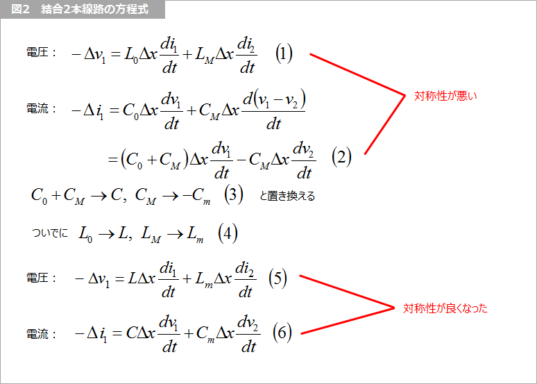
Figure 3 is an equivalent circuit using these symbols. Note that the coupling capacitance is negative.

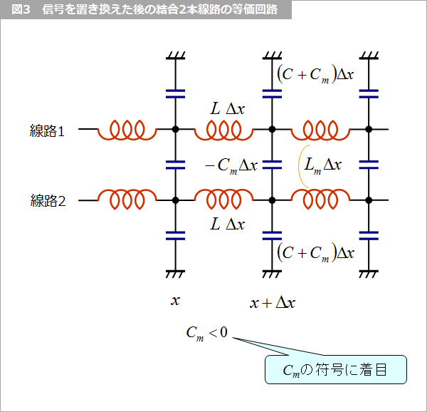
Figure 4 is a matrix representation of the equations, which also represents the capacitors and inductors in a matrix. Notice that the off-diagonal elements of the capacitor matrix have negative signs.

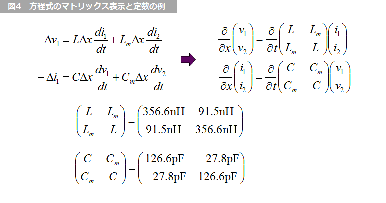
The capacitance between the lines is negative not only for two lines, but also for three or more coupled lines. Negative capacitance does not mean electrically negative like negative resistance, but it is just a conversion in terms of formulas. Therefore, it is possible to solve equations without such transformations, and I see many examples of doing so. However, I think that it is easier to convert and there are fewer mistakes.

How to find the line constant

These capacitors and inductors cannot be determined by simple formulas. In general, electromagnetic field analysis is performed based on the cross-sectional dimensions (2D) of the board. There are many software, but the following software that I use uses the Green's function.

Get parameters from section dimensions GreenExpress V2
* Due to the closure of Windward, we are unable to obtain the analysis tool GreenExpress V2.

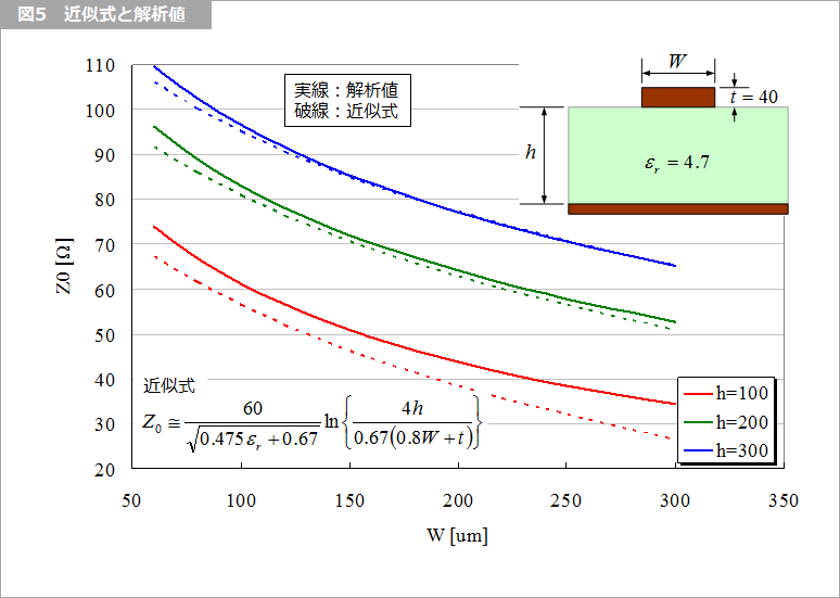
As shown in Figure 5, an approximation formula is sometimes used to obtain the characteristic impedance from the cross-sectional dimensions of the board. When this approximation formula was published, I think there was a condition for the range in which the approximation was valid, but there is a possibility that the approximation formula alone has taken on a life of its own. I don't have the literature at hand, so I can't confirm it, but I remember that it was a literature on microwaves in the 1960s.

Propagation constant of coupled line

These L and C constants can be used to describe the characteristic impedance and propagation delay, as shown in Figure 6. In two lines, there are two sets of characteristic impedance and propagation delay, called common mode and differential mode, respectively. (Footnote 1)

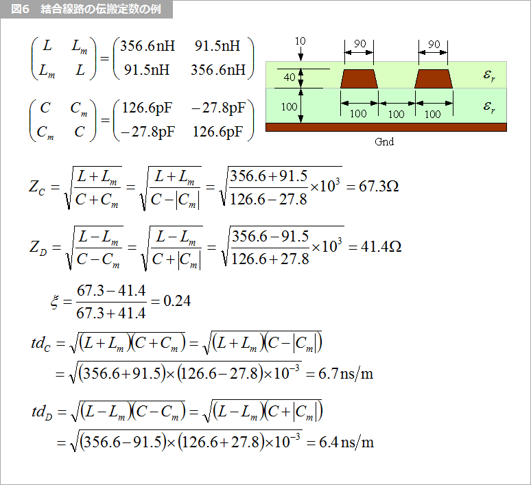
Denoting each mode with the initials C and D, the characteristic impedance and propagation delay are shown in Figure 6.

As mentioned earlier, Cm is negative, so the relationship between ZC and ZD is always ZC>ZD. The delay time is tdC=tdD on the middle (or inner) layers of the board, but tdC>tdD on the top (or outer) layers.

In "Exact Solution of Differential Crosstalk", Table 1 shows an example of four lines.

Footnote 1
The common mode is sometimes called the even mode or even mode, and the differential mode is similarly called the odd mode.