- 半導体事業HOME
- マクニカの製品・サービス
-
技術情報

-
イベント・セミナー
- 取扱メーカー
- サポート
- お問い合わせ
- 製品購入はこちら
- 半導体事業のメルマガ登録
![]()
![]() 条件を指定して絞り込む
条件を指定して絞り込む
現在2003件がヒットしています。check
トランジェント解析では、オシロスコープのように時間変化における信号レベルの確認ができます。 もし信号に含まれている周波数成分を確認したい際には、FFT機能を使うと便利です。信号の歪やノイズ成分をシミュレーションで確認することができます。
今回は、FFT機能についてご紹介させていただきます。
もしLTspiceを今から始められる方でしたら、以下の一覧から「基本編」を見ることをお勧めします。
また、基本的な回路の書き方から実行方法までを動画で見たいという方がいましたら、個人情報入力不要のオンデマンドセミナーがありますので、ご興味がありましたらぜひご覧ください。セミナーの詳細資料に関してもアンケートご記入の方に提供しています。
FFTとは?
FFT(Fast Fourier Transform)は、高速フーリエ変換のことです。
SPICEでは、スペクトルアナライザーのように信号に含まれている周波数成分とレベル(電力)を計算し表示します。FFT機能は、トランジェント解析(時間軸)で得られたデータを基にして計算を実行するので、Waveform Viewerに組み込まれている機能となります。
FFT機能を使ってみよう!
作業手順
今回は例題として、周波数と大きさが異なる3つの正弦波を合成した信号波形をトランジェント解析で確認し、FFT表示機能を使い周波数の分布を確認してみます。
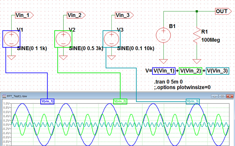
トランジェント解析の結果は、図2の通りです。
このOUT端子の波形を見るだけでは、周波数成分と大きさがわかりません。
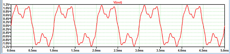
そこでFFT表示機能を使ってみます。
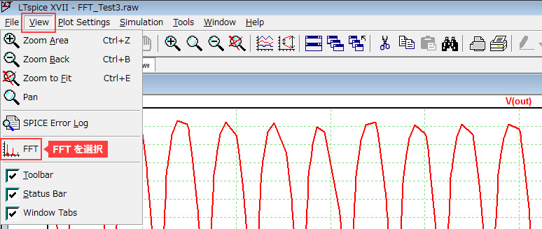
メニューバーからView→FFTを選択します。
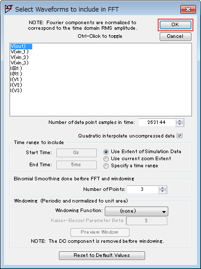
そうすると、図4のようなボックスがでてきますので、通常は「OK」をそのまま押してください。
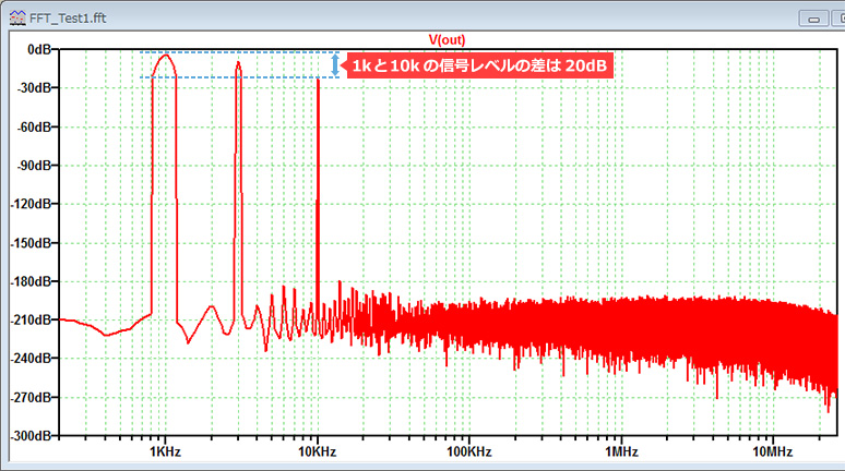
FFT表示結果は、図5のとおりです。
縦軸が信号レベル(dB)、横軸が周波数(Hz)の対数グラフが得られました。
周波数1kHz、3kHz、10kHzのところにピークがあり、波形の成分と大きさを把握することができました。
使い方のポイント
FFT機能を使う時は “.options plotwinsize=0” のコマンドを設定し解析データの圧縮を無効にすることを推奨します。このコマンドを使うことにより、ノイズフロアが低い結果が得られています(図5)。
またトランジェントコマンドの “Maximum Time Step” を信号の一周期の1/100よりも短くすると、良好なFFTの結果が得られます。ただし、短く設定するとシミュレーション時間が少しかかりますので、バランスをみて調整してください。
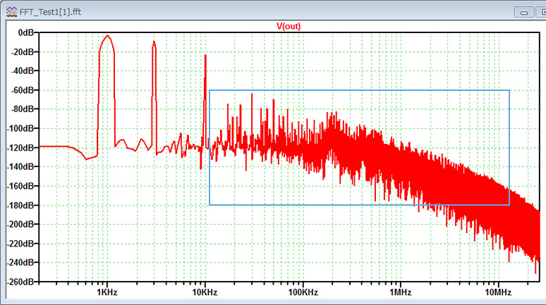
比較の為、.options でのplotwinsize指定を無くし、Maximum Time Stepもデフォルトのままでシミュレーションを実行しました。 先ほどの図5の結果と比較するとベースのノイズフロアが大きく、意図しない周波数でピークも見えています(図6)。
この結果からFFT解析では、“.options plotwinsize=0” のコマンドが重要であることを、ご理解頂けたかと思います。
電源ICの出力電圧信号をFFTで見てみよう!
以前、LTspiceを使ってみよう - DC-DCコンバータの動作確認 では、出力電圧のリップル電圧のレベルを確認しましたので、FFT機能で周波数成分も確認したいと思います。
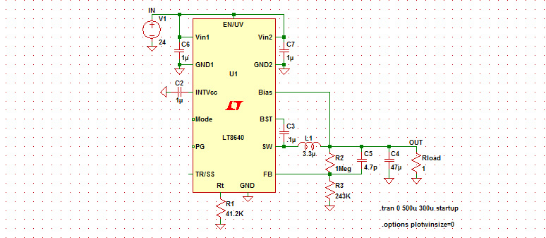
回路はLT8640のDemoファイルを使います。FFT解析では定常状態での結果が必要なため、電源が立ち上がった後のリプル電圧を確認します。そのためトランジェント解析のシミュレーション時間を500u~700usecにしました。
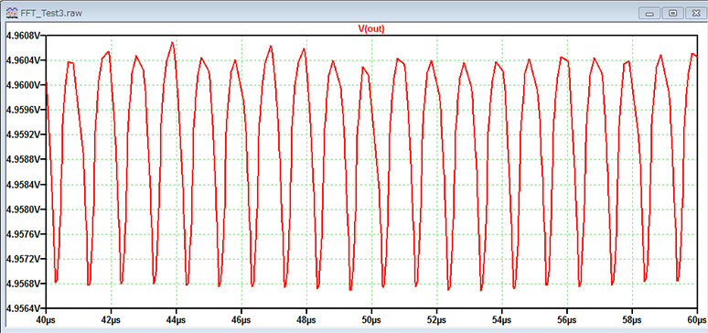
出力電圧のリップル波形は、図8の通りです。
FFT解析をすると、1MHzのスイッチング周波数成分だけでなく、2倍、3倍と偶数および奇数の周波数成分が含まれていることが確認できます(図9)。
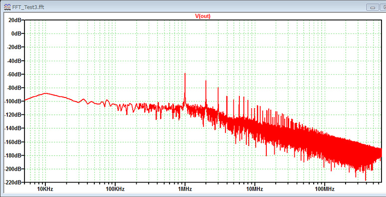
電源回路からのノイズは周辺回路やEMI試験に影響を与える場合があります。
FFT機能を使い周波数成分を把握することで、フィルタ設計などのノイズ対策をシミュレーションで検討することができます。
ぜひ、この機会にFFT機能を試してみてください!
今回検証したLTspiceデモ・ファイル
今回実施した2つのシミュレーションファイルが格納されています。ぜひお試しください!
最後に
今回はFFT機能をご紹介させていただきました!
まだLTspiceを使ったことがない方は、下記のリンクよりLTspiceをダウンロードしてみてください!
ぜひ、一度お試しください。
LTspiceのダウンロードはこちら
また、初心者向けのLTspiceセミナーも定期的に実施しています。LTspiceの基本操作を習得できますので、ご参加頂ければと思います。
LTspiceセミナーの情報はこちら
おすすめ記事/資料はこちら
記事一覧:LTspiceを使ってみようシリーズ
LTspice FAQ : FAQ リスト
技術記事一覧 : 技術記事
メーカー紹介ページ : アナログデバイセズ社
おすすめセミナー/ワークショップはこちら
お問い合わせ
本記事に関して、ご質問などありましたら以下よりお問い合わせください。
アナログ・デバイセズ メーカー情報Topへ
アナログ・デバイセズ メーカー情報Topに戻りたい方は以下をクリックしてください。